Week 1: Introduction to OLS Regression

Jesper Lindmarker

How did you find the previous course?

Week 1: Introduction to OLS Regression

🎓 Welcome to Week 1

Course: Statistics and Data Science II
Focus: Associations, regression, interpretation, and model intuition

🔍 Associations

• 🤔 Today we’ll start with associations. What does it mean?
• 🧠 Much of social science begins with a hypothesis about associations in the world:
  • Between 🎓 education and 💰 income, 📱 screen time and 😊 well-being, ⚧ gender and 💭 attitudes, or ⏱️ study time and 🧾 exam performance.
• ❤️ To make the content of this course meaningful, you need to connect it to your own interests.
  • What associations interest you? Take 1 minute to think ⏰.

✏️ Drawing Exercise

I want you to think about the association between hours studied and exam results for SDS-I.

• 📝 Task: On paper, sketch a scatterplot (points) of how you think these would be associated for you.
• The x-axis is the number of hours you studied for the SDS-I exam,
• The y-axis is your percentage of correct answers on the exam.

Associations

💬 Discussion

• How would you describe your sketched association?
• If you would connect your points, what is the shape of the line?

What Are We Really Asking?

• Would I have done better if I had studied more?
• Would someone else have done worse if they had studied less?
• Does studying cause better performance?

The Problem of the Missing Reality

We can imagine two possibilities for each student:

\[ Y_i(1) = \text{Exam score if student } i \text{ studies more} \] \[ Y_i(0) = \text{Exam score if student } i \text{ studies less} \]

These are called potential outcomes.

The Fundamental Problem of Causal Inference

For each student, we only observe one outcome:

• We see what happened, not what could have happened
• This missing data problem is what makes causality hard
• We cannot observe both \(Y_i(1)\) and \(Y_i(0)\).

So What Can We Do?

We can collect observed data:

• How many hours each student studied
• Their actual exam results

• From this we can look for patterns across individuals
  → This is the domain of statistical modeling

You Already Made a Hypothesis

Earlier you imagined your own points of potential outcomes on a scatterplot.

Put together, these plots form a collective hypothesis about the relationship between:

• Study time
  
• Exam performance
• The next task would be to test it with data.

What is Regression?

Regression is a way to model the relationship between variables.

• Predict an outcome (Y), often called the dependent variable.
• Use one or more predictors (X), often called our indepedent variable(s)
• We can use it to make predictions 🎯

Predict y

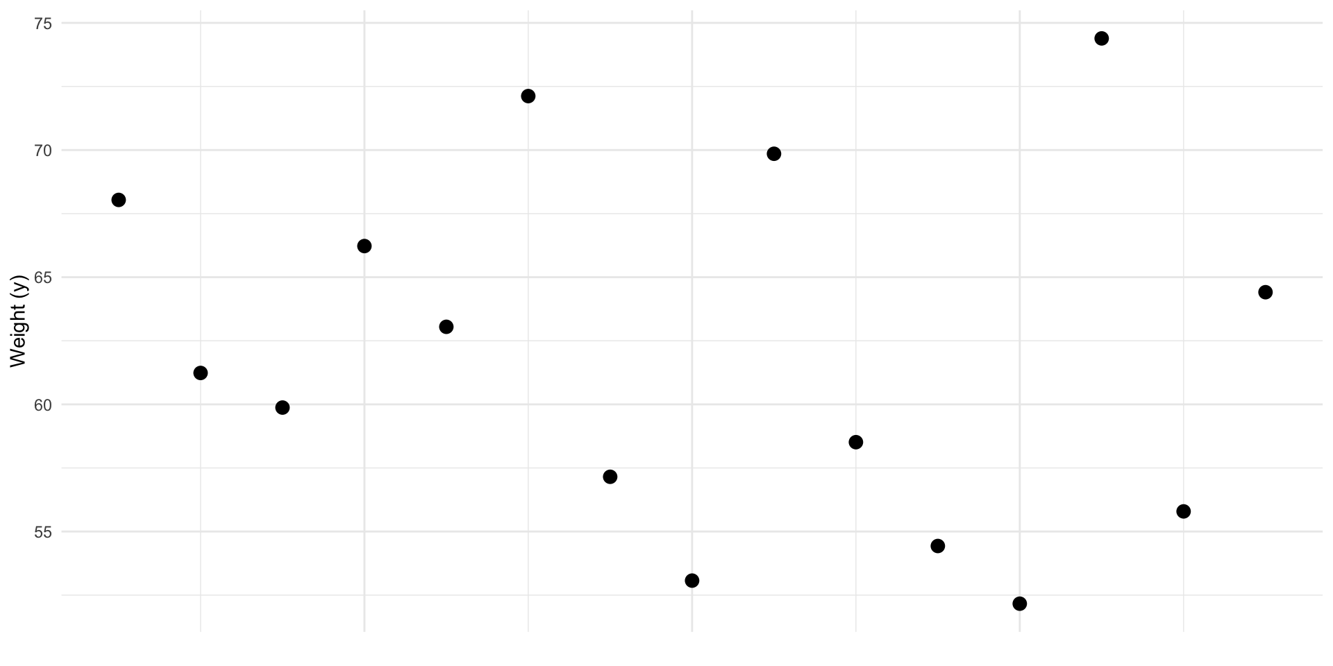
Given this data. What’s our best prediction of a new \(y_i\)?

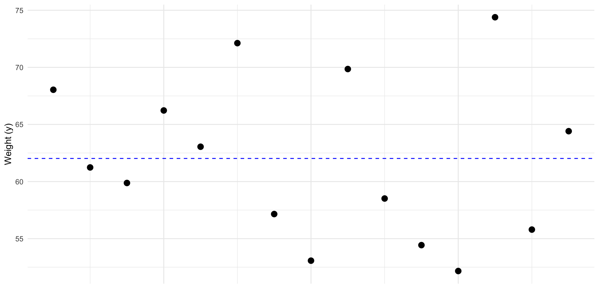
Predict y

The best prediction for a new \(y\), is the mean: \(\bar y\). In other words \(\widehat y = \bar y\)

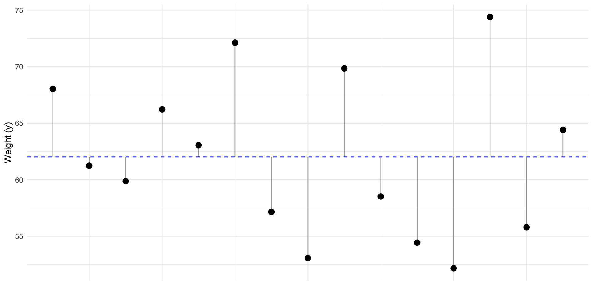
Predict y

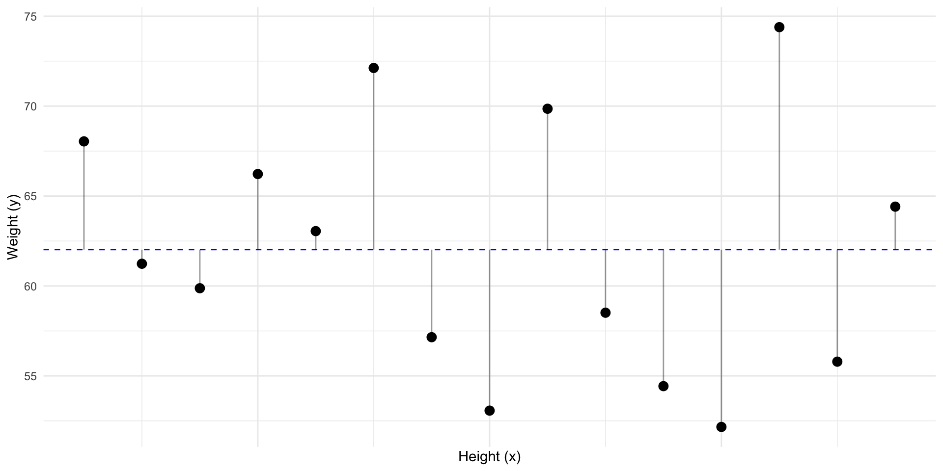
So how “wrong” would we be if we had predicted \(\bar y\) for every \(y_i\)?

Predict y

These “errors” are called residuals (\(residual_i = y_i - \widehat{y}_i\))

Predict y

Given no other information, guessing \(\bar y\) minimizes the residuals.

Predict y

But, what if we have some other information?

Predict y

Can we make a better prediction of \(y\) using \(x\)?

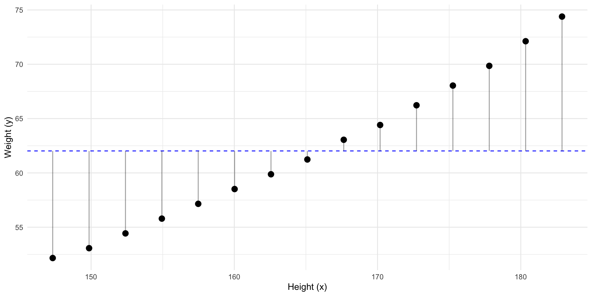
Predict y

If we sort by that information…

Predict y

Can we improve our best guess of \(y\)?

Predict y

Can we draw a straight line with less residuals?

Predict y

Can we draw a line with less residuals?

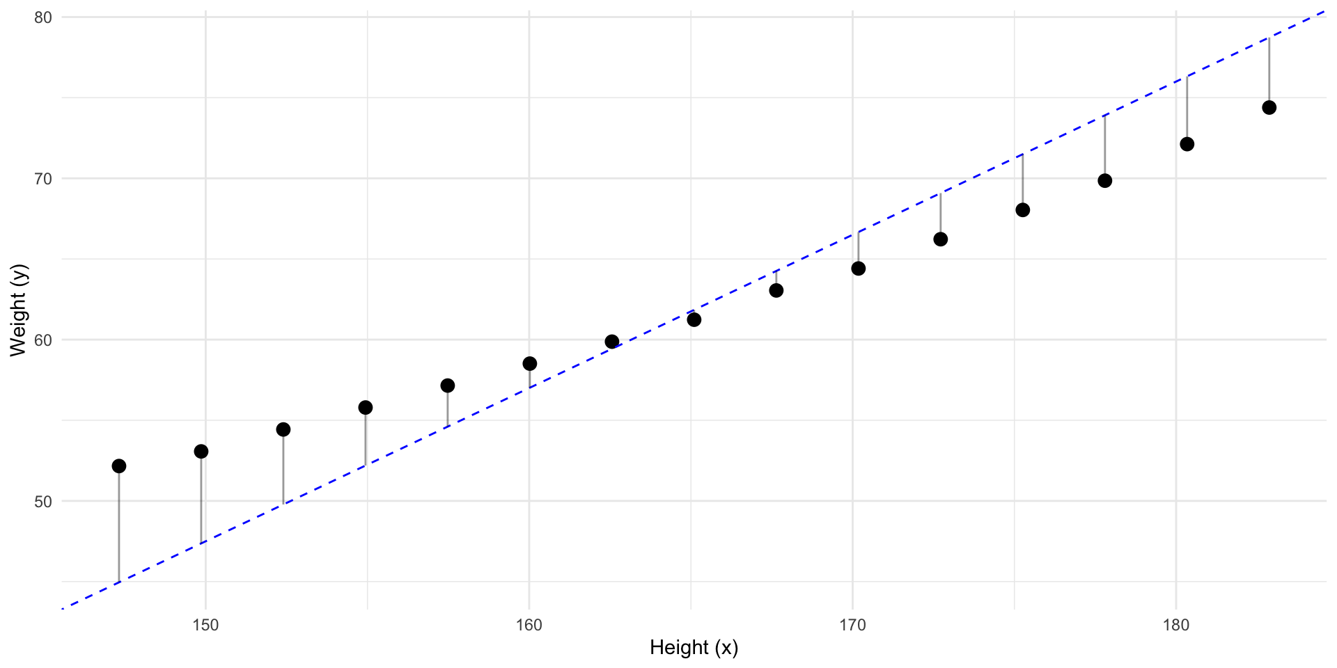
Predict y using x

Better! But what line has the least residuals?

Predict y using x

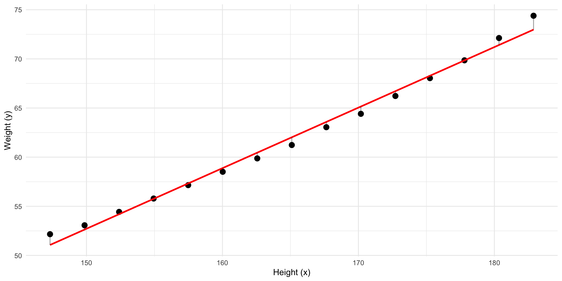
This line has the least residuals. It’s a regression line.

Predict y using x

We have fitted a model to our data.

• The model predict \(y\) using \(x\)
• This means that if we know a \(x\) we can calculate the model’s prediction of \(y\)
• It’s a representation of the association between the variables in our data.
• Currently it’s in the form of a straight line equation

The straight line equation

\[ y = a + b \cdot x \] Where:

• \(a\) is the intercept

• \(b\) is the slope

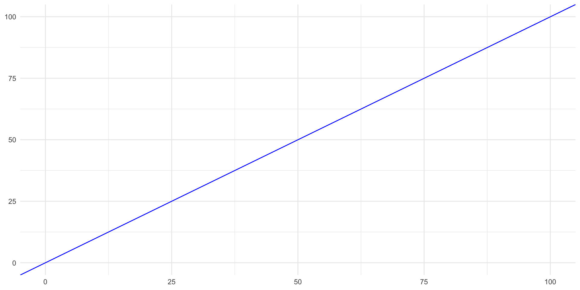
A Simple Example

\[ y = 0 + 1 \cdot x \]

• If \(x = 2\), then \(y =\)?
• \(2\)
• If \(x = 10\), then \(y =\)?
• \(10\)

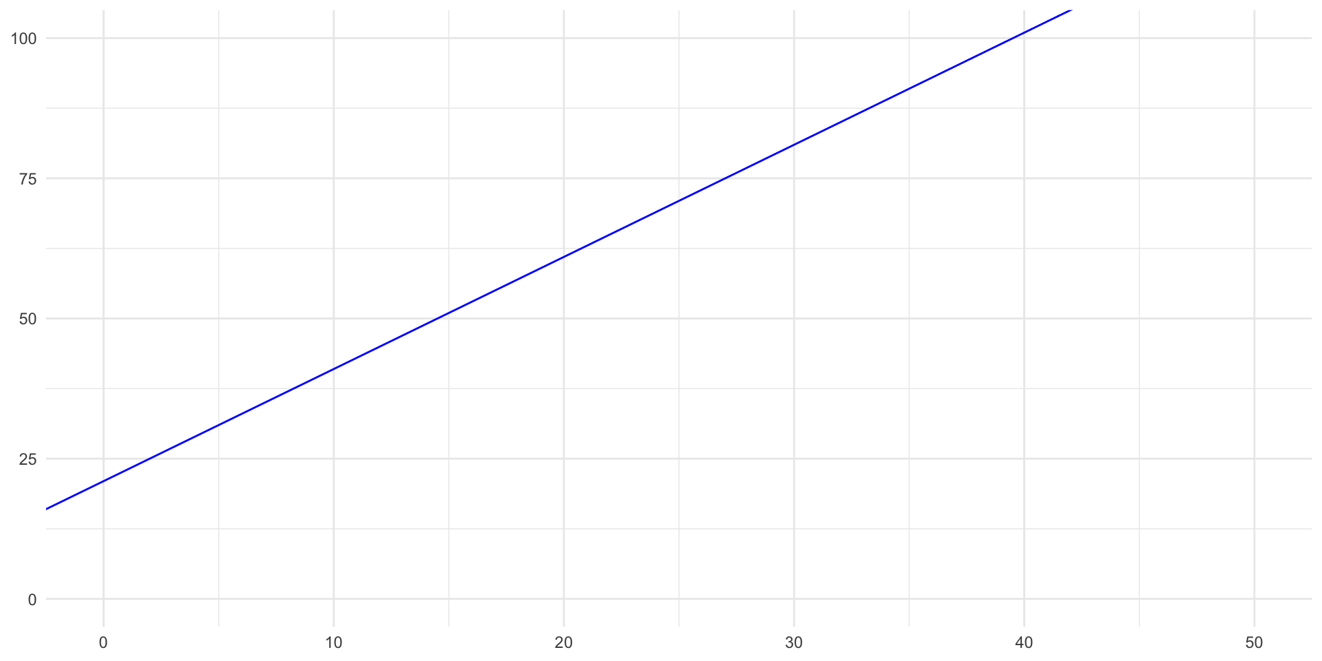
Another

\[ y = 21 + 2 \cdot x \]

• If \(x = 0\), then \(y =\)?
• \(21\)
• If \(x = 10\), then \(y =\)?
• \(41\)

Our Model Equation

\[ \widehat{y} = -39.7 + 0.62 \cdot x \]

• If \(x = 160\), then \(y = ?\)
  • \(y = 58.5\).
• If height increases by 1 cm, how much would predicted weight increases by?
  • \(0.62kg\)
  • The slope tells us how \(y\) changes when \(x\) increases by one unit.
• What would be the predicted weight of someone with \(0\) height?
  • \(-39.7kg\)

Our Model Equation

summary(mod)

Call:
lm(formula = weight ~ height, data = women)

Residuals:
    Min      1Q  Median      3Q     Max 
-0.7862 -0.5141 -0.1739  0.3364  1.4137 

Coefficients:
             Estimate Std. Error t value Pr(>|t|)    
(Intercept) -39.69694    2.69296  -14.74 1.71e-09 ***
height        0.61610    0.01628   37.85 1.09e-14 ***
---
Signif. codes:  0 '***' 0.001 '**' 0.01 '*' 0.05 '.' 0.1 ' ' 1

Residual standard error: 0.6917 on 13 degrees of freedom
Multiple R-squared:  0.991, Adjusted R-squared:  0.9903 
F-statistic:  1433 on 1 and 13 DF,  p-value: 1.091e-14

Let’s stop and summarise

With a regression, we can describe a pattern between variables in our data — like height and weight — using a mathematical model, like a straight line.

• We have quantified an association.
• This might represent some “real” association in the “real” world.

What is our assumed model?

But the real-world is messy:

• Two people with the same height might weigh different amounts.
• There are many factors we don’t measure or can’t explain.
• Our data might be off.
• It is why we get residuals

We can write this as an assumed model:

\[ Y_i = \beta_0 + \beta_1 X_i + \varepsilon_i \]

Understanding the model

\[ Y_i = \beta_0 + \beta_1 X_i + \varepsilon_i \]

• \(Y_i\) and \(X_i\) are random variables (population level)
• \(\beta_0 + \beta_1 X_i\): the systematic part — recognize the straight line?
• \(\varepsilon_i\): the unsystematic part — the error.

From Model to Prediction

From our sample, we estimate:

\[ \widehat{y}_i = \hat{\beta}_0 + \hat{\beta}_1 x_i \]

• \(x_i\): observed weight for individual \(i\)
• \(\widehat{y}_i\): our predicted height for individual \(i\)
• \(\hat{\beta}_0\): estimated intercept. \(\hat{\beta}_1\): estimated slope.
• \(r_i = y_i - \widehat{y}_i\): the residual — how far off our prediction was

To summarize

• Observed Data: \((x_i, y_i)\) — what we actually see

• Assumed Model: \(Y_i = \beta_0 + \beta_1 X_i + \varepsilon_i\)

  • includes error \(\varepsilon_i\) (unknown, unobserved)

• Fitted Model: \(\widehat{y}_i = \hat{\beta}_0 + \hat{\beta}_1 x_i\)

  • produces residuals \(r_i = y_i - \widehat{y}_i\) (known, measurable)

So:

• The assumed model is a hypothesis about how \(Y\) might relate to \(X\)
• The fitted model describes the data and “fits” the model
• Residuals ≠ Errors — but both reflect imperfect predictions

How Good Is Our Fit? Or, goodness of fit

How much better is our model than just guessing the mean?

• Remember the “guessing” we did using only \(y\)?
• We use that as the total sum of residuals to “explain”, or the total variance to explain.
• Then we compare that to the sum of residual amount of residuals in our model.

Squared Residuals

Remember, this is how we defined residuals: \(r_i = y_i - \widehat{y}_i\)

However, when we compare models, we use squared residuals: \(r_i^2 = (y_i - \widehat{y}_i)^2\)

• It makes all values positive
• Penalized large errors more (\(4^2 = 16\) is way worse than \(2^2 = 4\))
• Optimization becomes easier.

Sum of Squares

• We add up (sum) all of the now squared residuals from the baseline model: \(\sum (y_i - \bar{y}_i)^2\)

• Then we sum the squared residuals from our model: \(\sum (y_i - \widehat{y}_i)^2\)

Sum of Squares

• Baseline model: \[ \text{Total Sum of Squares (TSS)} = \sum (y_i - \bar{y})^2 \]
• The model: \[ \text{Residual Sum of Squares (RSS)} = \sum (y_i - \widehat{y}_i)^2 \]
• Share of total variance explained by our model (\(R^2\)): \[ R^2 = 1 - \frac{\text{RSS}}{\text{TSS}} \]

Introducing \(R^2\)

We define:

\[ R^2 = 1 - \frac{\text{RSS}}{\text{TSS}} \]

• \(R^2\) is the proportion of variation explained by the model
• Always between 0 and 1:
  • \(R^2\) = 0: model is no better than just guessing the mean
  • \(R^2\) = 1: perfect prediction

Regression constellations

OLS - Ordinary Least Squares

• What we have discussed is commonly called OLS regression
• It estimates parameters with the “least squares”
• In other words: OLS finds the line that minimizes the sum of squared residuals.

But When Is This Valid?

We’ve learned:

• How to fit a regression line
• How to interpret it
• How to evaluate its fit using \(R^2\)

But regression only works well if certain conditions are met.

These are the assumptions of OLS.

OLS Assumptions

OLS Assumption 1: Linearity

• The linearity assumption means that the expected value of Y is a linear combination of known functions of the predictors.
• The model must be linear in the parameters, but not necessarily in the raw variables.

✅ Valid: \(Y = \beta_0 + \beta_1 X + \beta_2 X^2\)

❌ Invalid: \(Y = \beta_0 + \sin(\beta_1 X)\)

• ⚠️ What might cause violations: model misspecification or omitted variables that introduce non-linear structure in the residuals.
• 🔧 Try adding polynomial terms, more controls, interactions, or transforming variables.

OLS Assumption 2: Independence

• Observations must be independent of one another.
• If observations are related as in repeated measures, grouped/clustered data (e.g., students in schools), or time series, then standard errors will be incorrect.

• ⚠️ What might cause violations: clustered designs, panel or time-series data, or spillover effects where one observation influences another.
• 🔧 Use cluster-robust SEs, multilevel models, or time-series adjustments.

OLS Assumption 3: Constant Variance (Homoscedasticity)

• The spread of residuals should be roughly constant across all levels of X.
• If the spread increases or decreases, the model errors are heteroscedastic.
• 🔍 Check using residual vs. fitted plots — funnel shapes = violation.

• ⚠️ What might cause violations: omitted variables that affect variance (e.g., income level affecting outcome variability), or scale effects where larger values have naturally larger errors.
• 🔧 Use robust SEs or transform Y (e.g., log-scale).

OLS Assumption 4: Normality of Errors

• The residuals should be approximately normally distributed.
• This matters most in low-n studies when making inferences (e.g., confidence intervals, hypothesis tests).
• 📈 Use a histogram or Q–Q plot of residuals to check.
• 🧪 Doesn’t affect point estimates, but does affect statistical tests.

• ⚠️ What might cause violations: outliers, skewed dependent variables, or incorrect functional form.
• 🔧 Consider trimming outliers, or change functional form.

Summary: OLS Assumptions

• Linearity: Relationship can be expressed with linear predictors
  
• Independence: Observations are unrelated
  
• Homoscedasticity: Equal spread of residuals
  
• Normality: Residuals follow a normal distribution (low \(n\))
  

• OLS is robust to mild violations, especially in large samples — but you should know how to diagnose and how they affect interpretation.

• We’ll revisit these in the lab later.

Interactive visualization of OLS

https://setosa.io/ev/ordinary-least-squares-regression/

What are your questions? ✋

See you at the lab! 🌶️