Week 2: Multiple Regression

Jesper Lindmarker

How difficult was last week?

Asking Questions in Swedish Higher Education

• Asking questions shows engagement and curiosity, not weakness.
  
• It will never affect your grade
• It’s only the parts specified in the study guide that affects your grade.

💬 Questions are welcome:

• During lectures and labs
• By email

🧠 Remember:
Swedish academic culture values independent thinking and open dialogue.

Learning is a collaboration, not a one-way transmission.

Week 2: Multiple Regression

Welcome to Week 2

Topic: Multiple Regression, Categorical Variables

Goal: Extend our regression toolkit

🔁 Week 1 Recap: Simple Linear Regression

We learned how to:

• Simulate and visualize linear relationships

• Fit models like:
  

• \(Y = \beta_0 + \beta_1 X + \varepsilon\)

• Interpret coefficients:

  • \(\beta_1\) = how much Y changes when X increases by 1 unit

• Diagnose assumptions

• Understand \(R^2\) and residuals

• 🧠 Example: “How does the number of hours studied relate to exam score?”

🗺️ What We’ll Talk About Today

This week, we’re moving beyond simple models with just one variable.

We’ll explore:

1. Multiple regression
   👉 How to include more than one independent variable

2. Controlling for other factors
   👉 How to separate the effect of one variable from the influence of others

3. More interpretation
   👉 How to interpret significance, uncertainty and importance

4. Categorical variables
   👉 What to do when your variable isn’t continous but categorical — like field of study or gender

Multiple regression

🧮 Note on Terminology: The Regression Coefficient

In Lecture 1, we called it the slope of the line.
In statistics, it’s also called β (beta), the regression coefficient, or sometimes the parameter estimate.

Symbol / Name	Also called…
\(\beta_0\)	intercept, constant, baseline
\(\beta_1\)	slope, coefficient, association, effect, weight
\(b\)	(alternate symbol)

🧮 Note on Terminology: Variables

When talking about variables in regression, we also have different terms.

Role in model	Also called…
Outcome	dependent var, response, Y
Predictor	independent var, explanatory var, X, treatment
Other predictors	covariates, controls, features
Error	residual, disturbance, noise

🧮 Note on Terminology: Variables

🧠 Key idea:
We’re modeling how Y depends on X, possibly while adjusting for other variables.

💡 You’ll hear different terms depending on:

• The field (statistics, sociology, economics…)

• The goal (describe patterns, prediction, causal inference…)

🤔 Why Add More Predictors?

We usually add more variables for one of two reasons:

✅ Prediction
👉 To build models that can accurately guess the outcome for new cases, even if we don’t fully understand why (You will cover this more in the ML course)

✅ Inference
👉 To build better models for understanding patterns — or to get closer to causal effects

In social science, inference often means:

• Describing relationships more accurately

• Testing theories about how things are connected

• Sometimes estimating causal effects (when possible)

• Different goals = different reasons to expand the model.

🔍 Better Predictions

• Predictors explain different parts of the variation in our outcome (\(y\))
• This means: Smaller residuals -> Higher \(R^2\)

🧩 Main challenge: Use some of the data to “train” and then predict on another.

Where might we value prediction?

• 🏥 Medicine: Predict cancer survival based on age, treatment, tumor stage
• 📊 Policy: Who is most at risk of long-term unemployment?
• 🧠 Theory Testing: Prediction as the ultimate test of a theory
• 💳 Marketing: Who is likely to buy based on age, income, past behavior?
• 🤖 Machine Learning: Predict the next word (like GPT!)

🎯 Inference

In social science, we often care about the effect of one variable on another.

🧠 Some classic questions:

1. Does education reduce crime?
2. Do parental incomes shape children's educational outcomes?
3. Does neighborhood context affect life chances?
4. Does social media use cause depression?
5. Does immigration impact native wages?
6. Do marriage and family structure affect child development?
7. Does unemployment lead to worse health?
8. Does gender bias affect hiring decisions?
9. Does access to early childhood education improve long-term outcomes?
10. Does political messaging change voter behavior?

But…

• Very few things in life are caused by just one factor

🧩 Other explanations

1. Does education reduce crime?
   👉 Maybe people with higher education also had better childhood environments

2. Do parental incomes shape children’s outcomes?
   👉 Or is it parental education that matters more?

3. Does social media cause depression?
   👉 Or are people who are already struggling more drawn to social media?

4. Does unemployment lead to worse health?
   👉 Or do people in worse health become unemployed more often?

5. Does gender bias affect hiring decisions?
   👉 Could industry or applicant background explain part of it?

🎯 This is why we build multivariate models:
To separate overlapping influences and make more credible inferences.

🧩 Other explanations

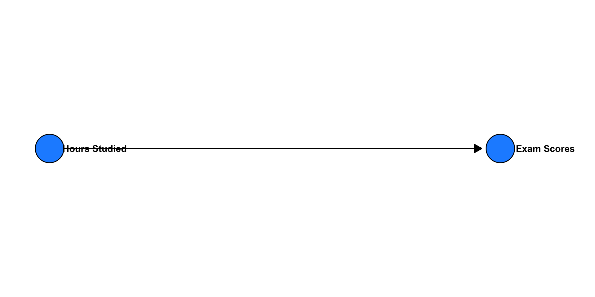
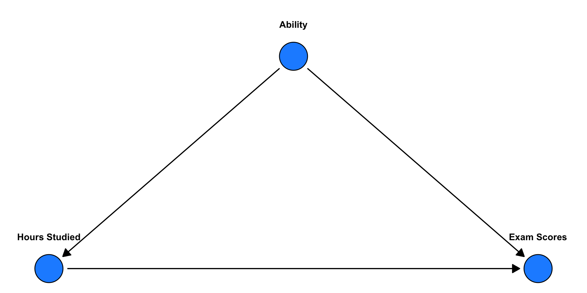
🧠 So what about the classic question: Does more hours studying increases students’ exam scores? — What else might matter?

(Causal graph)

🧩 Other explanations

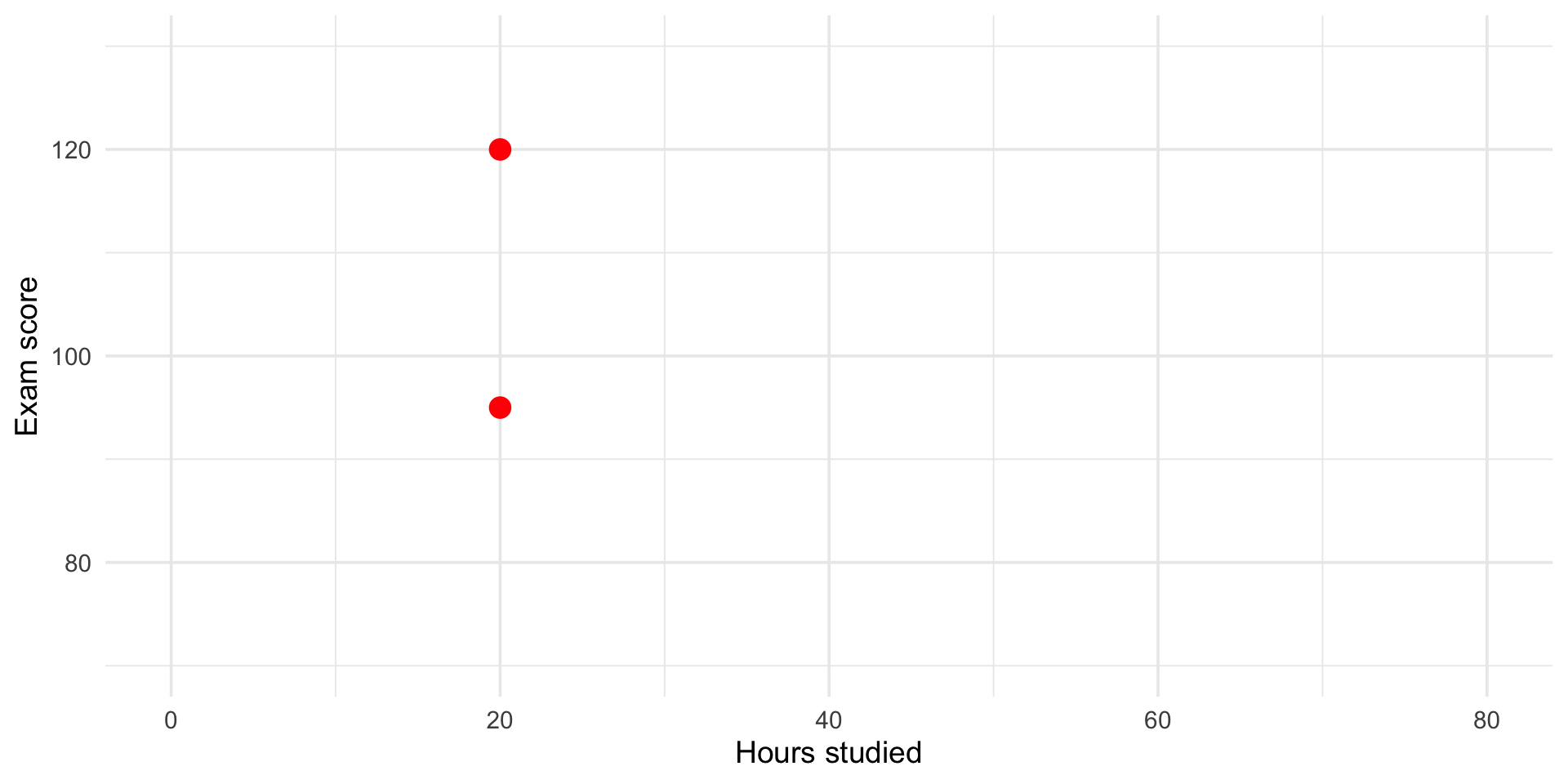
Two students both study 20 hours for the exam.
But they get different scores.
Why?

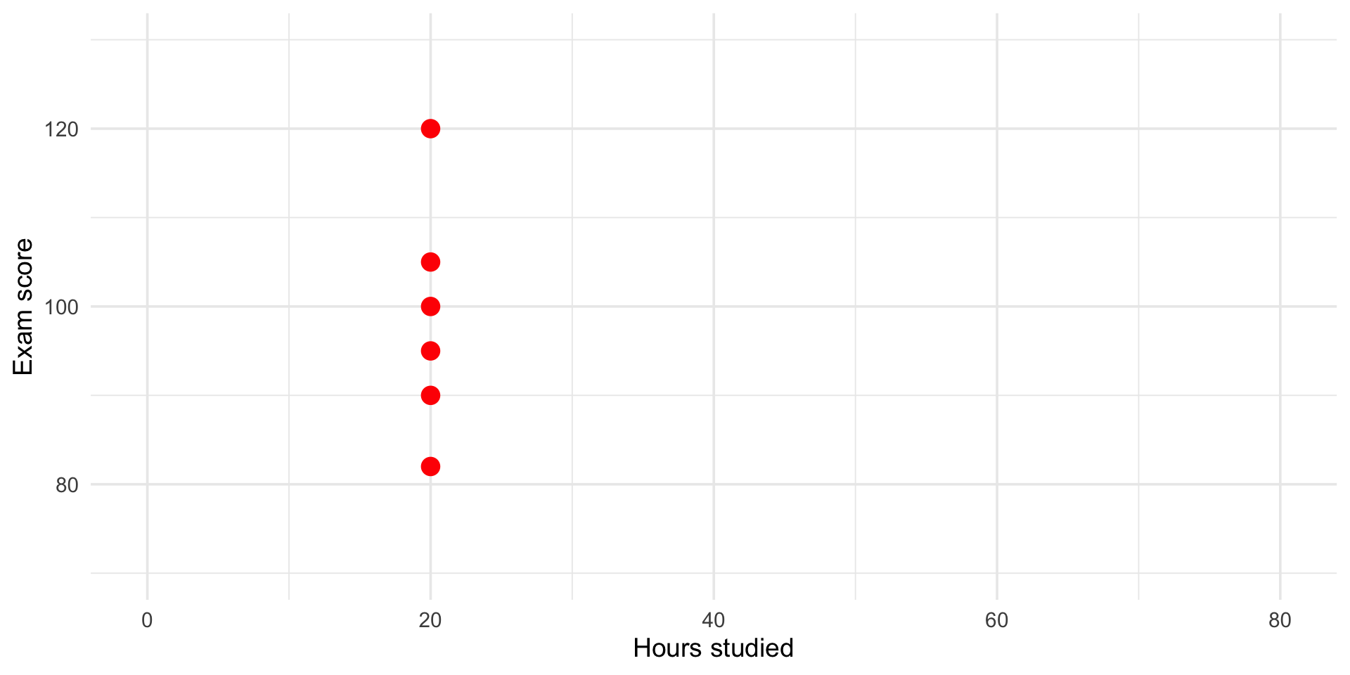
🧩 Other explanations

Many students both study 20 hours for the exam.
But they get different scores.
This represents more variance to be explained

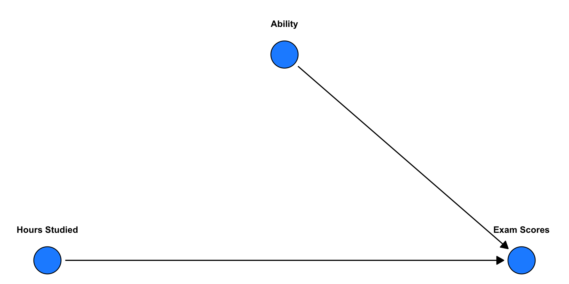
🧩 Other explanations

🧠 So what about the classic question: Does more hours studying increases students’ exam scores? — What else might matter?

Let’s look at the data!

head(data2, n = 15)

   exam_score hours_studied previous_gpa
1         116          26.2           84
2         106          33.0           60
3         123          51.5           NA
4         123          42.6           93
5         117          35.4           89
6         116          53.8           72
7         112          62.9           90
8         124          57.7           77
9         112          62.2           60
10        123          41.0           52
11        121          76.3           96
12        134          54.3           86
13        113          45.0           63
14        103          25.4           67
15        127          62.7           80

Let’s look at the data!

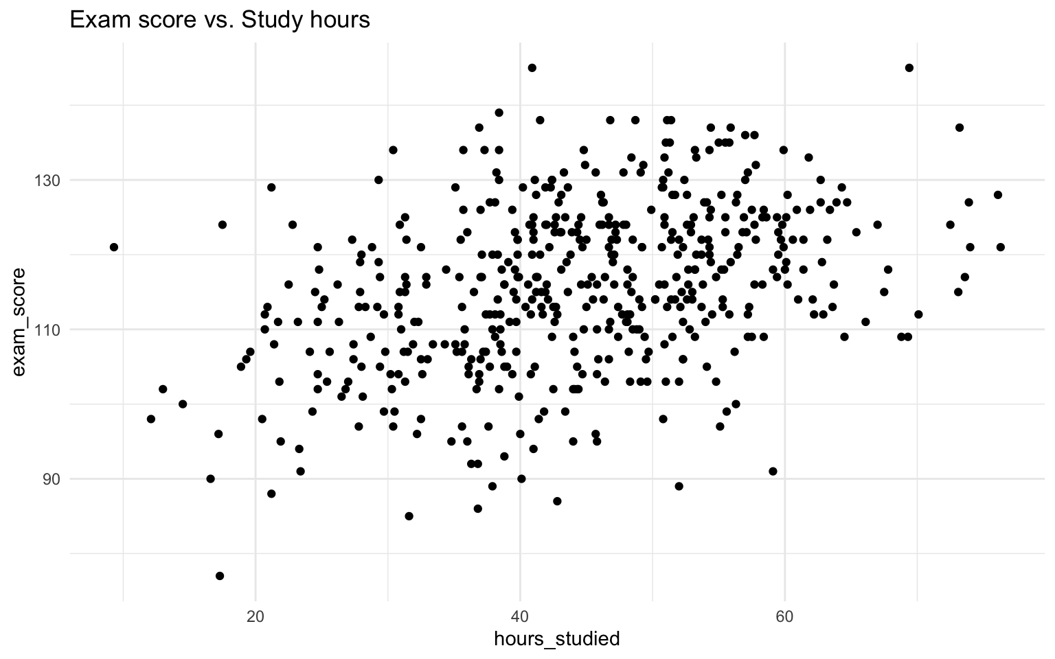
Let’s look at the data!

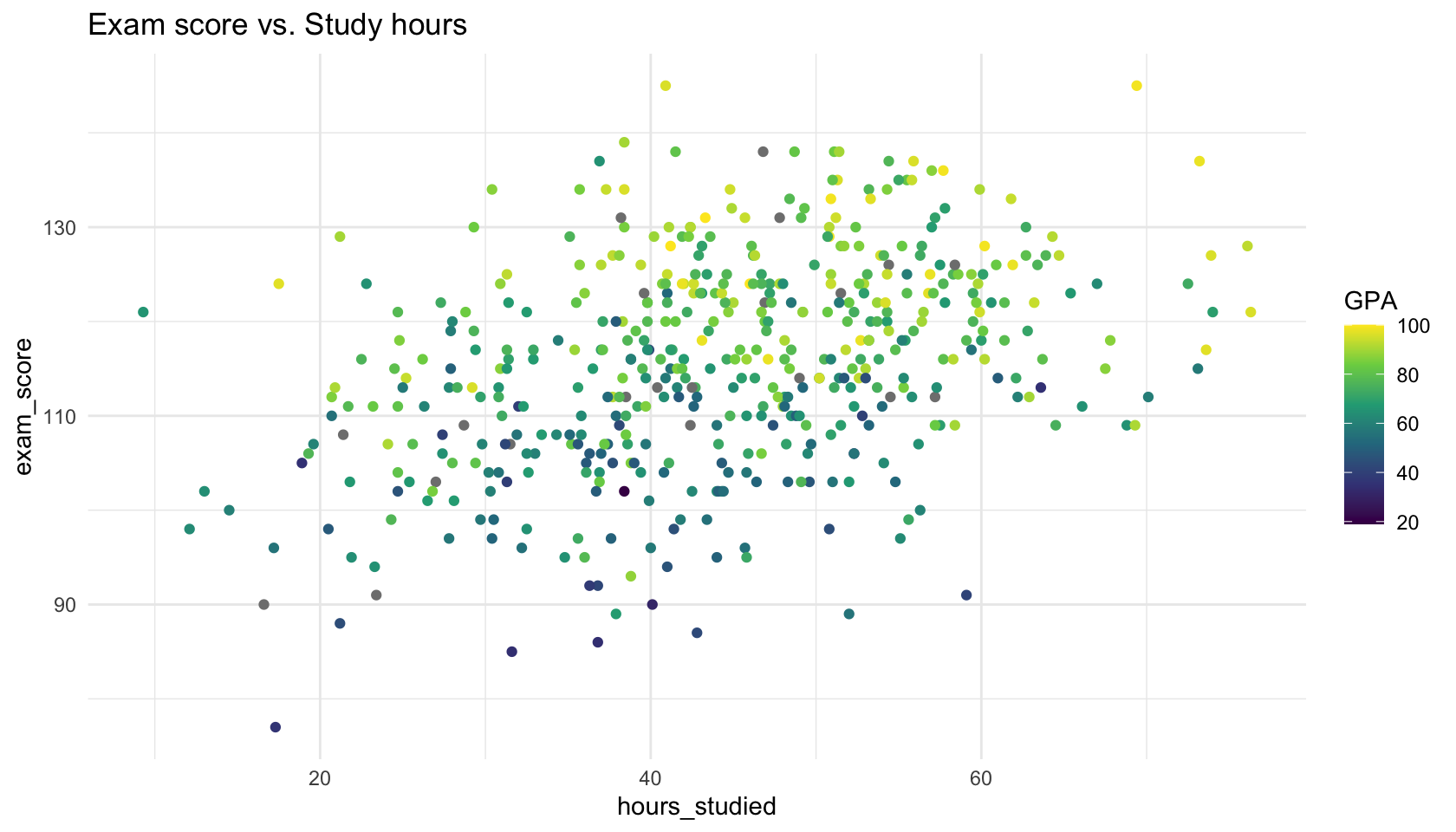
🎯 What is the Correct Comparison?

When we ask,

“Does studying more increase exam scores?”

we have to be careful who we compare.

• If we compare students with different GPA, part of the difference in scores may be due to ability, not studying.
  
• What we really want is to compare students who are similar in GPA, but differ in hours studied.
  

💡 This is, when working correctly, what multiple regression does —
it let’s us ask: Among students with the same GPA, does more studying predict higher exam scores?

Multiple Regression Model

\[ Y = \beta_0 + \beta_1 X_1 + \beta_2 X_2 + \varepsilon \]

• Each coefficient captures the independent effect of a variable
• We say that we control for the other variable
• Interpretation is ceteris paribus — all else held constant
• We still interpret the marginal effect: “When \(X_1\) increases by one unit, Y change, on average by \(\beta_1\)…”
• But now we must add to our interpretation: “…all else held constant”

Multiple Regression Model

mod <- lm(exam_score ~ hours_studied + previous_gpa, data = data)

Call:
lm(formula = exam_score ~ hours_studied + previous_gpa, data = data)

Residuals:
     Min       1Q   Median       3Q      Max 
-27.7000  -5.5333   0.1781   5.3906  26.0899 

Coefficients:
              Estimate Std. Error t value Pr(>|t|)    
(Intercept)   76.52935    2.06180   37.12  < 2e-16 ***
hours_studied  0.21293    0.03212    6.63 9.21e-11 ***
previous_gpa   0.40806    0.02486   16.41  < 2e-16 ***
---
Signif. codes:  0 '***' 0.001 '**' 0.01 '*' 0.05 '.' 0.1 ' ' 1

Residual standard error: 8.218 on 471 degrees of freedom
  (26 observations deleted due to missingness)
Multiple R-squared:  0.4503,    Adjusted R-squared:  0.448 
F-statistic: 192.9 on 2 and 471 DF,  p-value: < 2.2e-16

• How do we interpret these results?

Multiple Regression Model

For a general estimated model:

\(\widehat{y} = \widehat{\beta}_0 + \widehat{\beta}_1 x_1 + \widehat{\beta}_2 x_2\)

Correct OLS Coefficient Interpretation

“Within the observed data, a one-unit increase in \(x_1\) is associated with an average change of \(\widehat{\beta}_1\) units in \(y\), holding all other included variables constant.

The estimated coefficient has a standard error of [SE] and p-value = [p-value]. At a significance level of \(\alpha\) = 0.05, this effect is [statistically significant / not significant].

This reflects an association, not necessarily a causal effect, and the interpretation depends on the assumptions of the linear model.”

Another phrasing

“When comparing two cases that are alike in all other included predictors, the one with a 1-unit higher value of \(x_1\) is predicted to have \(\widehat{\beta}_1\) higher \(y\), on average.”

Multiple Regression Model

For our model:

\(\widehat{\text{exam_score}} = 76.53 + 0.21 \times \text{hours_studied} + 0.41 \times \text{GPA}\)

Correct OLS Coefficient Interpretation

Within the observed data, and conditional on the variables included in the model, a one-unit increase in hours studied is associated with an average change of 0.21 points in exam score, holding previous GPA constant.

The estimated coefficient has a standard error of 0.03 and p-value = \(<0.001\). At a significance level of \(\alpha\) = 0.05, this effect is statistically significant.

This reflects an association, not necessarily a causal effect, and the interpretation depends on the assumptions of the linear model.

Another phrasing

“When comparing two people with the same level of GPA, the one who studied one hour more is predicted to have 0.21 higher exam score, on average.”

Multiple Regression Model

For our model:

\(\widehat{\text{exam_score}} = 76.53 + 0.21 \times \text{hours_studied} + 0.41 \times \text{GPA}\)

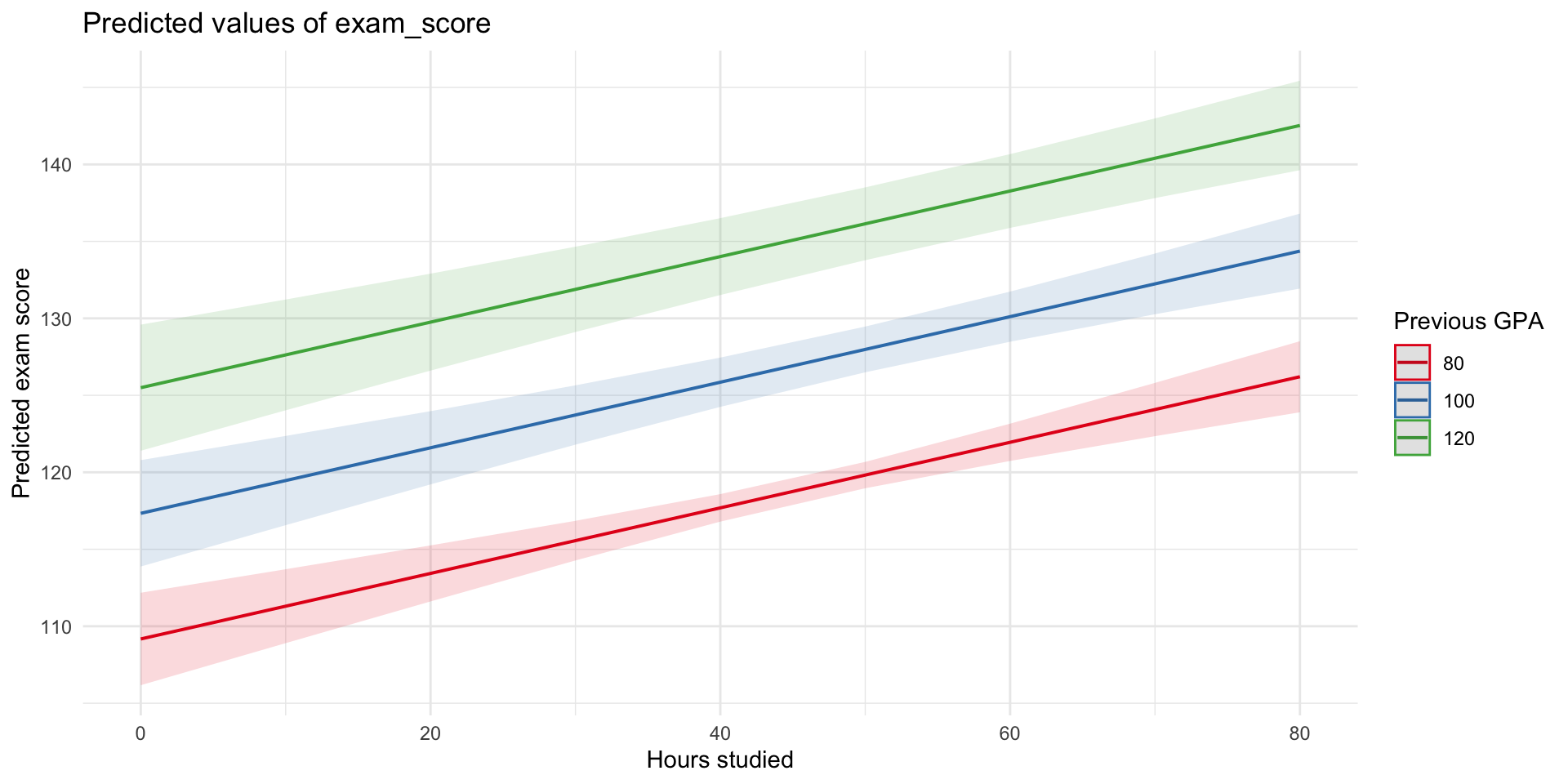
• We can use our model equation to make predictions of hypothetical people:
  • Let’s imagine someone with a GPA of 100 who studied 0 hours:
  • \(\widehat{\text{exam score}} = 76.53 + 0.21\times 0 + 0.41 \times 100 = 117.3\)
  • or someone with a GPA of 120 who studied 30 hours:
  • \(\widehat{\text{exam score}} = 76.53 + 0.21\times 30 + 0.41 \times 120 = 131.9\)

We can also plot the predictions

library(ggeffects)
pred_plot <- ggpredict(mod, terms = c("hours_studied", "previous_gpa [80, 100, 120]"))

plot(pred_plot) + labs(
    x = "Hours studied",
    y = "Predicted exam score",
    color = "Previous GPA",
  ) + theme_minimal()

What Does “Controlling For” GPA Mean?

Terminology Alert

In regression, controlling for, adjusting for and accounting for all mean the same thing

➡️ We include one or more variables in the model to isolate the unique effect of the independent variable, holding the rest constant.

• Repetition: Why did we wish to control for GPA?

  • We know hours studied is related to exam results — students who study more tend to do better
  • We also know GPA is related — stronger students often perform better.
  • Therefore, we have to control for GPA in our model and thus compare students with similar GPA but different hours studied

🤔 But Wait…

• What if students with higher GPA also tend to study more?

Then:

• Some of the variation in exam scores explained by hours studied might be better explained by GPA.
• This overlap is called shared variance and is a source of confounding
• So what is confounding?

🤔 Confounding

🧐 Question: If we don’t control for GPA, what might be wrong with the estimated \(\beta\) for hours studied?

• It will be overestimated, i.e. too large. In other words, biased.

🎯 The Problem of Confounding

If two predictors (like GPA and hours studied) are correlated, and both relate to the outcome…

• We might over- or underestimate the role of studying if we don’t control for GPA.
• This is known as confounding — a third variable (GPA) that influences both our predictor (studying) and our outcome (exam scores).
• In other words, a common cause

✅ Multiple regression helps us adjust for this and estimate the unique contribution of each variable.

🧩 Confounding is a subtle and complex issue — often oversimplified. We’ll return to it later in the course.

Why the Coefficient Changes

Model	Coefficient on hours_studied
lm(exam_score ~ hours_studied)	Picks up total association
lm(exam_score ~ hours_studied + previous_gpa)	Association holding GPA constant

➡️ The meaning of coefficients depends on what’s in the model

📊 Interpreting coefficients, p-values, and Confidence Intervals

📊 Interpreting coefficients, p-values, and Confidence Intervals

When we run a regression, we get estimates for our coefficients (the slopes) —
but we also get uncertainty measures.

Call:
lm(formula = exam_score ~ hours_studied + previous_gpa, data = data)

Residuals:
     Min       1Q   Median       3Q      Max 
-27.7000  -5.5333   0.1781   5.3906  26.0899 

Coefficients:
              Estimate Std. Error t value Pr(>|t|)    
(Intercept)   76.52935    2.06180   37.12  < 2e-16 ***
hours_studied  0.21293    0.03212    6.63 9.21e-11 ***
previous_gpa   0.40806    0.02486   16.41  < 2e-16 ***
---
Signif. codes:  0 '***' 0.001 '**' 0.01 '*' 0.05 '.' 0.1 ' ' 1

Residual standard error: 8.218 on 471 degrees of freedom
  (26 observations deleted due to missingness)
Multiple R-squared:  0.4503,    Adjusted R-squared:  0.448 
F-statistic: 192.9 on 2 and 471 DF,  p-value: < 2.2e-16

These tell us how confident are we that this relationship exists in the population?

🎯 What the p-value Tells Us

• The p-value quantifies how surprising our data would be if there were actually no effect.

💬 In words:

If the true β were 0, what is the probability of seeing an effect at least this big (or bigger) just by chance?

🧠 Small p-value → our data are unlikely under the “no effect” world.
This suggests that the relationship in our sample probably reflects a real pattern.

🚫 But remember:

• p < 0.05 ≠ “the effect is large”
• p > 0.05 ≠ “there is no effect”
• p-values are about evidence, not importance.

📏 What the Confidence Interval Tells Us

confint(mod)

                   2.5 %     97.5 %
(Intercept)   72.4778929 80.5808054
hours_studied  0.1498233  0.2760388
previous_gpa   0.3591984  0.4569131

The 95% confidence interval gives a range of plausible values for the true coefficient.

💬 In words:

“If we repeated this study many times, 95% of the calculated intervals would contain the true β.”

• Narrow interval → we estimated the effect precisely
  
• Wide interval → we are less sure of the effect size
  

If the CI does not include 0 (the null hypothesis value), the effect is statistically significant at the 5% level (same idea as p < 0.05).

💡 Substantive Significance – Does It Matter?

Even when an effect is statistically significant,
we should still ask: Is it meaningful?

Statistical significance → The effect is unlikely to be zero.
Substantive (practical) significance → The effect is large enough to matter in the real world.

💬 Example:

If studying one extra hour raises exam scores by 0.23 points,
this may be statistically significant — but is it educationally important?

• Would that difference change a grade, a decision, or a policy?
  
• Does it represent a meaningful impact in the real context?

🧠 From Significance to Substance

Statistical ≠ Substantive significance.
Always interpret size and context — not just stars and p-values ⭐️

✅ Always report and discuss:

• Direction — Is the effect positive or negative?
  
• Magnitude — How big is it?
  
• Uncertainty — How certain is it?
  
• Meaning — Why does it matter in real terms?

🎯 Goal: Move beyond “Is it significant?”
toward “Is it important?”

🧩 Putting It All Together

Predictor	Estimate	95% CI	Interpretation
Hours studied	0.23	[0.17, 0.30]	For each additional hour studied, exam score increases by 0.23 points, on average, holding GPA constant. The confidence interval (95%) does not contain 0 and the estimate is therefore signicant on the p<0.05 level. In substantive terms… ???
GPA	0.41	[0.36, 0.46]	-

📈 Adjusted R²

Call:
lm(formula = exam_score ~ hours_studied + previous_gpa, data = data)

Residuals:
     Min       1Q   Median       3Q      Max 
-27.7000  -5.5333   0.1781   5.3906  26.0899 

Coefficients:
              Estimate Std. Error t value Pr(>|t|)    
(Intercept)   76.52935    2.06180   37.12  < 2e-16 ***
hours_studied  0.21293    0.03212    6.63 9.21e-11 ***
previous_gpa   0.40806    0.02486   16.41  < 2e-16 ***
---
Signif. codes:  0 '***' 0.001 '**' 0.01 '*' 0.05 '.' 0.1 ' ' 1

Residual standard error: 8.218 on 471 degrees of freedom
  (26 observations deleted due to missingness)
Multiple R-squared:  0.4503,    Adjusted R-squared:  0.448 
F-statistic: 192.9 on 2 and 471 DF,  p-value: < 2.2e-16

📈 Adjusted R²

Adjusted \(R^2\) is a goodness-of-fit measurement that accounts for the number of predictors in the model.

• \(R^2\) always increases (or stays the same) when you add more predictors,
  even if they’re not meaningful.
• Adjusted R² corrects for this by penalizing model complexity.
• Use Adjusted \(R^2\) when:
  • Comparing models with different numbers of predictors.
  • Evaluating the balance between fit and parsimony.

Example

Adding irrelevant predictors may raise R² from 0.80 → 0.82,
but Adjusted R² might drop from 0.79 → 0.78 — signaling that they don’t provide much to the model.

Categorical Variables

Categorical Variables

In the world of data, not all variables are numeric.
Sometimes we want to include a categorical independent variable like:

• 🧑‍🎓 Field of study (e.g., Humanities, Social Sciences, Natural Sciences)
  
• 🌍 Region or country
• 📅 Day of the week

Example: Field of Study

data %>% count(field)

        field   n
1  humanities 155
2 natural_sci 181
3  social_sci 164

In our data, we have a variable with three categories:

• Humanities
  
• Social Science
  
• Natural Science

• which we can use as an independent variable in a regression: exam_score ~ field

Categorical Variables: Intuition

Regression interprets categorical variables as group differences.

• The intercept tells us the average for the reference group
• Coefficients tell us how much higher/lower the outcome is compared to that group

Let’s Try It

mod3 <- lm(exam_score ~ field, data = data)
summary(mod3)

Call:
lm(formula = exam_score ~ field, data = data)

Residuals:
    Min      1Q  Median      3Q     Max 
-36.123  -7.167  -0.123   7.701  29.701 

Coefficients:
                 Estimate Std. Error t value Pr(>|t|)    
(Intercept)      113.1226     0.8827 128.151  < 2e-16 ***
fieldnatural_sci   5.1758     1.2027   4.303 2.03e-05 ***
fieldsocial_sci    2.1762     1.2311   1.768   0.0777 .  
---
Signif. codes:  0 '***' 0.001 '**' 0.01 '*' 0.05 '.' 0.1 ' ' 1

Residual standard error: 10.99 on 497 degrees of freedom
Multiple R-squared:  0.03656,   Adjusted R-squared:  0.03269 
F-statistic: 9.431 on 2 and 497 DF,  p-value: 9.553e-05

• ✅ This estimates the difference in exam score by field of study
  
• ✅ Baseline = Humanities

Interpreting Categorical Coefficients

mod3 <- lm(exam_score ~ field, data = data)
coef(summary(mod3))

                   Estimate Std. Error    t value     Pr(>|t|)
(Intercept)      113.122581  0.8827322 128.150503 0.000000e+00
fieldnatural_sci   5.175762  1.2027056   4.303432 2.026106e-05
fieldsocial_sci    2.176200  1.2311257   1.767650 7.773291e-02

• Intercept = Average exam score for Humanities students
• Social Science = Difference from Humanities
  
• Natural Science = Difference from Humanities

🧠 These are group means, but shown as a regression!

Visualize the Group Differences

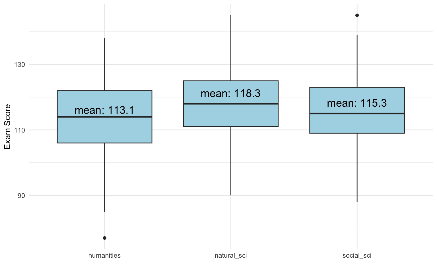
This is exactly what the regression captures.

Dummy Variables

• Dummy variables can be seen as a special case of categorical variable which only has two categories: 0 and 1.

• Gender is coded as a dummy in our data:

data %>% count(gender)

  gender   n
1      0 250
2      1 231
3     NA  19

• 0 = Male
  
• 1 = Female

Let’s add gender to our model

mod4 <- lm(exam_score ~ field + gender, data = data)
summary(mod4)

Call:
lm(formula = exam_score ~ field + gender, data = data)

Residuals:
    Min      1Q  Median      3Q     Max 
-35.499  -7.123   0.623   7.735  30.623 

Coefficients:
                 Estimate Std. Error t value Pr(>|t|)    
(Intercept)       112.499      1.021 110.210  < 2e-16 ***
fieldnatural_sci    4.765      1.226   3.886 0.000117 ***
fieldsocial_sci     1.878      1.259   1.491 0.136679    
gender              1.859      1.004   1.851 0.064752 .  
---
Signif. codes:  0 '***' 0.001 '**' 0.01 '*' 0.05 '.' 0.1 ' ' 1

Residual standard error: 10.99 on 477 degrees of freedom
  (19 observations deleted due to missingness)
Multiple R-squared:  0.03917,   Adjusted R-squared:  0.03312 
F-statistic: 6.481 on 3 and 477 DF,  p-value: 0.0002635

• Dummy variables always use 0 as the reference.
• Question: What is the meaning of the intercept?

Interpretation Reminder

For dummy variables:

• Coefficient = group difference
  
• Intercept = baseline group

“Compared to male students in Humanities…”

Let’s add hours studied

mod5 <- lm(exam_score ~ field + gender + hours_studied, data = data)
summary(mod5)

Call:
lm(formula = exam_score ~ field + gender + hours_studied, data = data)

Residuals:
    Min      1Q  Median      3Q     Max 
-33.345  -6.466   0.619   6.784  28.102 

Coefficients:
                 Estimate Std. Error t value Pr(>|t|)    
(Intercept)      96.80829    1.90189  50.901  < 2e-16 ***
fieldnatural_sci  5.41889    1.12727   4.807 2.06e-06 ***
fieldsocial_sci   1.91996    1.15575   1.661   0.0973 .  
gender            0.91916    0.92796   0.991   0.3224    
hours_studied     0.35869    0.03822   9.384  < 2e-16 ***
---
Signif. codes:  0 '***' 0.001 '**' 0.01 '*' 0.05 '.' 0.1 ' ' 1

Residual standard error: 10.02 on 471 degrees of freedom
  (24 observations deleted due to missingness)
Multiple R-squared:  0.1931,    Adjusted R-squared:  0.1863 
F-statistic: 28.18 on 4 and 471 DF,  p-value: < 2.2e-16

• Question: What is the meaning of the intercept?

🎯 Back to prediction

Call:
lm(formula = exam_score ~ field + gender + hours_studied, data = data)

Residuals:
    Min      1Q  Median      3Q     Max 
-33.345  -6.466   0.619   6.784  28.102 

Coefficients:
                 Estimate Std. Error t value Pr(>|t|)    
(Intercept)      96.80829    1.90189  50.901  < 2e-16 ***
fieldnatural_sci  5.41889    1.12727   4.807 2.06e-06 ***
fieldsocial_sci   1.91996    1.15575   1.661   0.0973 .  
gender            0.91916    0.92796   0.991   0.3224    
hours_studied     0.35869    0.03822   9.384  < 2e-16 ***
---
Signif. codes:  0 '***' 0.001 '**' 0.01 '*' 0.05 '.' 0.1 ' ' 1

Residual standard error: 10.02 on 471 degrees of freedom
  (24 observations deleted due to missingness)
Multiple R-squared:  0.1931,    Adjusted R-squared:  0.1863 
F-statistic: 28.18 on 4 and 471 DF,  p-value: < 2.2e-16

Let’s predict the exam score for…

1. A man, with a background in humanities, who studied 10h.
2. A woman, with a background in natural science, who studied 20h.

🧠 Week 2 summary

🔍 What You Should Understand

• Why we model
  Regression helps us understand how variables relate
  → “All else held constant” is the key logic

• What we estimate
  Each coefficient as a partial association
  → change in Y for a one-unit change in X, holding others constant

• What can go wrong
  Omitting confounders bias our results
  

• How to interpret results
  Look at
  → Direction (+/−)
  → Magnitude (how large?)
  → Uncertainty (CI / p-value)
  → Meaning (does it matter?)

🧩 What You Should Learn To Do

✅ Fit and interpret multiple regression models
lm(y ~ x1 + x2)
Understand coefficients, p-values, and confidence intervals

✅ Explain confounding and why we control for variables
→ Compare like with like

✅ Include categorical predictors
→ Intercept = reference group
→ Coefficients = group differences

✅ Move beyond significance
→ Focus on substance and context

⭐ Big Picture:
Multiple regression lets us separate overlapping causes
and move from association → credible inference.

🎯 Next Week:
Interactions & non-linearity — when effects depend on something else 🌀