Week 3: Interactions, non-linearities and transformations

Jesper Lindmarker

How difficult was last week?

Week 3: Interactions, non-linearities and transformations

From Week 2 — “All else held constant”

Last week we learned to:

Add more predictors to explain more of the variation in \(Y\)
Control for confounders to isolate the unique effect of each variable
Interpret coefficients while holding everything else constant
Include categorical variables as group differences (dummy or factor variables)

🧠 But note: Our models so far assumed that studying one more hour helps all students equally.

➡️ This week, we’ll challenge that idea.

What if the effect of studying depends on who you are
or on how much you already study?

✏️ Drawing Exercise

Again, I want you to think about the association between hours studied and exam results for SDS I.

Now imagine two groups:
- Students who partied the night before the exam 🍻
- Students who did not party 😇

📝 Task:
- On paper, sketch one scatterplot with different shapes for the 🍻 and the 😇.
- The x-axis is hours studied
- The y-axis is percent correct answers on the exam

💬 Discussion

What differences did you draw?

Did both groups have the same average score?
Did both groups have the same slope?
Who benefits most from studying?

➡️ This idea — that a relationship differs across groups —
is the foundation of interaction effects.

Interactions/moderation: Effects That Depend on Other Variables

Sometimes the effect of one variable depends on the level of another.

💡 This is called an interaction or moderation.

Example:

Does studying help everyone equally?
Or do some things affect the usefulness of one hour of studying?

Interaction/moderation vs. confounding

🧠 Why is this important?

Much of social science asks whether an association is stronger or weaker for different groups:

Does the return to education differ between men and women?
Does neighborhood context matter more for low-income families?
Does social media use affect teens more than adults?

➡️ These are all interaction questions.

Intuition for Interactions

If two students study the same amount, but one was out partying the night before the exam.

Can they make use of their hours studied to the same extent?
Or, does the lack of sleep change how useful studying is?
In other words: Does the effect of studying depend on partying/sleeping well?

➡️ If there is an interaction, the slopes should be different for those how partied and those who did not

Visualizing an Interaction

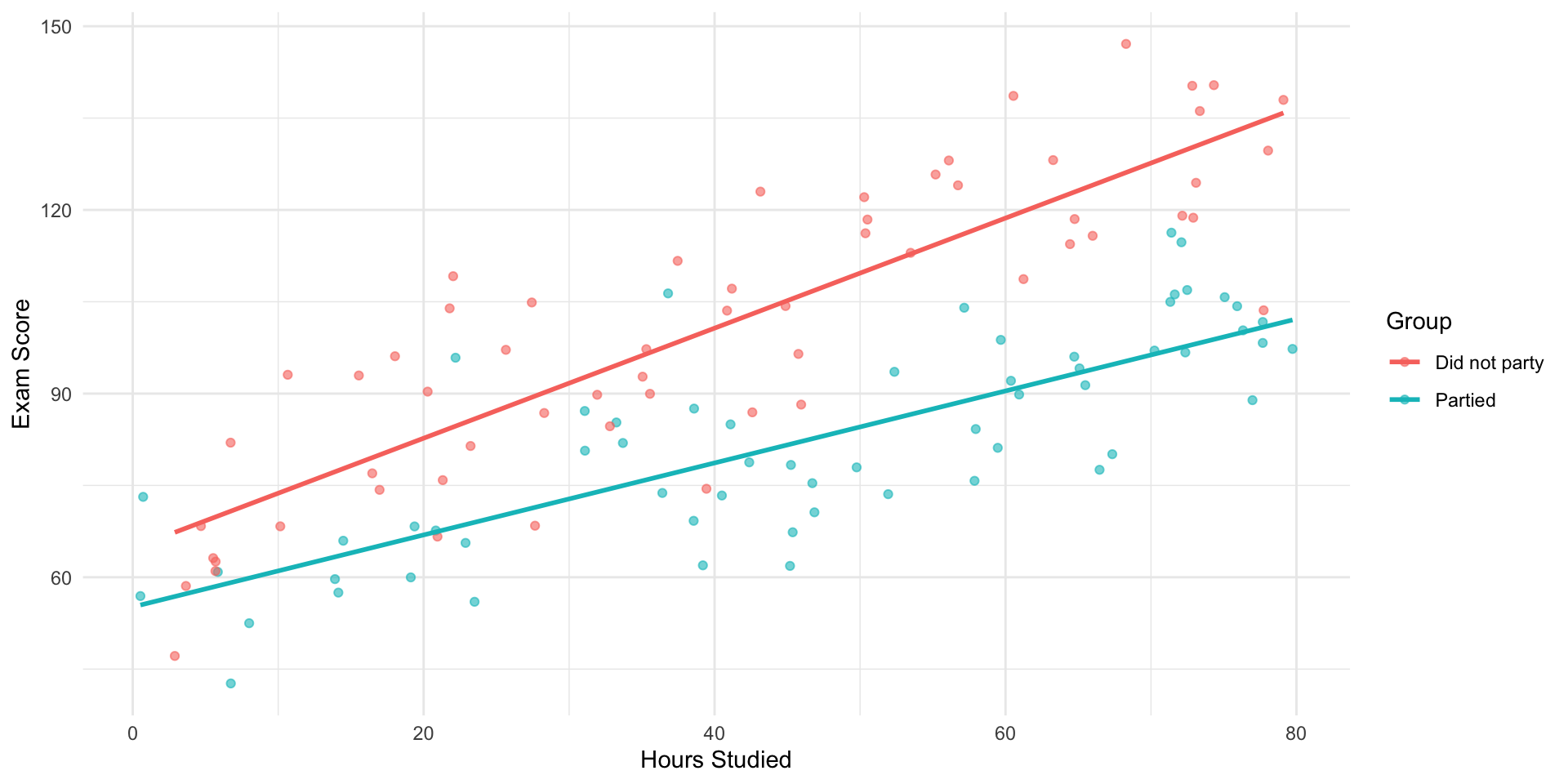
What is the marginal effect of one hour more studying?

🧩 Stratified Models

We could simply fit separate regressions by stratifying the data:

results_noparty <- lm(exam_score ~ hours_studied, data = filter(data, party_hard == "No"))
results_party <- lm(exam_score ~ hours_studied, data = filter(data, party_hard == "Yes"))

That’s what the plot currently shows
✅ This adjusts for the stratfied variable
✅ And it allows different slopes

⚠️ But there are drawbacks with stratifying

You can’t easily test statistically if slopes differ.
You lose sample size and efficiency.
You can’t include continuous moderators easily.

💡 Solution: use a single regression with an interaction term.

Interaction Term in a Regression

\[ y = \beta_0 + \beta_1 x_1 + \beta_2 x_2 + \beta_3 (x_1 \times x_2) \]

\(\beta_3\) is the interaction coefficient
Mathematically, the interaction is a multiplication of the variables
Interpretation becomes significantly more difficult
Important rule: When you have an interaction, all lower order terms must be included

R-syntax for this is

lm(y ~ x1 + x2 + x1:x2, data = ...)

or using shorthand:

lm(y ~ x1 * x2, data = ...)

Fit a Model with an Interaction

Let’s include an interaction between hours_studied and previous_gpa:

mod_interaction <- lm(exam_score ~ hours_studied * previous_gpa, data = data)
summary(mod_interaction)


Call:
lm(formula = exam_score ~ hours_studied * previous_gpa, data = data)

Residuals:
    Min      1Q  Median      3Q     Max 
-27.956  -5.675   0.125   5.385  26.147 

Coefficients:
                            Estimate Std. Error t value Pr(>|t|)    
(Intercept)                67.848588   6.747162  10.056  < 2e-16 ***
hours_studied               0.417420   0.151585   2.754  0.00613 ** 
previous_gpa                0.525405   0.092194   5.699 2.18e-08 ***
hours_studied:previous_gpa -0.002731   0.002018  -1.353  0.17661    
---
Signif. codes:  0 '***' 0.001 '**' 0.01 '*' 0.05 '.' 0.1 ' ' 1

Residual standard error: 8.227 on 452 degrees of freedom
Multiple R-squared:  0.4508,    Adjusted R-squared:  0.4472 
F-statistic: 123.7 on 3 and 452 DF,  p-value: < 2.2e-16

How to Interpret This?

\[ \widehat{\text{Exam Score}} = \beta_0 + \beta_1 \times \text{Hours} + \beta_2 \times \text{GPA} + \beta_3 \times (\text{Hours} \times \text{GPA}) \]

\(\beta_0\): Predicted exam score when Hours Studied = 0 and GPA = 0
\(\beta_1\): Effect of studying if GPA = 0
\(\beta_2\): Effect of GPA if studying = 0
\(\beta_3\): How much the effect of one predictor changes for each one-unit increase in the other.
- When interpreting, start with the direction of the interaction (+/-)

🧠 In our data, with a negative interaction coefficient, this means: The higher their GPA, the less studying adds to exam score.

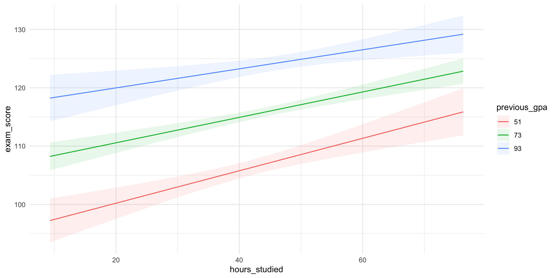
Let’s Plug in Some Values

\[ \widehat{\text{Exam Score}} = 67.85 + 0.42 \times \text{Hours} + 0.53 \times \text{GPA} + (-0.0027) \times (\text{Hours} \times \text{GPA}) \]

Now let’s calculate the effect of 1 more hour studied, at different GPA levels

We don’t need the full equation — just the parts that change when we increase study time by 1 hour:

\[ \widehat{\text{Exam Score}} = 0.42 \cdot 1 + (-0.0027)\times (1 \times \text{GPA}) \]

At different values of GPA:

  GPA                  Calculation Effect_of_Study
1  40 0.42 + (-0.0027 × 40) = 0.31            0.31
2  60 0.42 + (-0.0027 × 60) = 0.25            0.25
3  80  0.42 + (-0.0027 × 80) = 0.2            0.20

These are the marginal effects — the estimated effect of studying one more hour at each GPA level.
Importantly, it’s not constant but varies depending on GPA.

Marginal effect of hours studied

We’ve calculated the marginal effect at a few GPA levels. Now let’s compute and plot it across all values using the marginaleffects package.

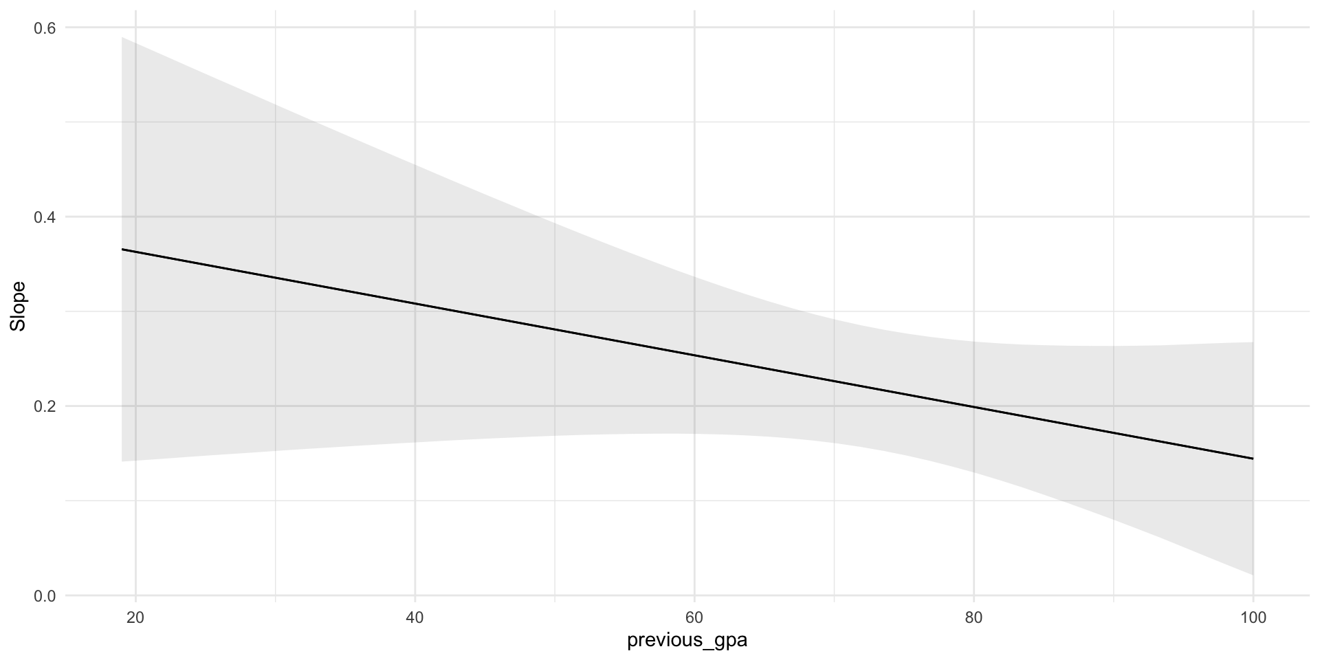
Predictions Visualized

Using the marginaleffects package.

Understanding Marginal Effects

In regression, the marginal effect of a variable tells us:

How much the outcome (\(y\)) changes when one predictor (\(x\)) increases by one unit, holding all other variables constant.

In a simple OLS model, the marginal effect is just the coefficient (\(\beta_1\)).
In more complex models, e.g. interactions, the marginal effect is no longer constant, we have to calculate it for different values of other variables.
👩🏽‍🔧 Slightly more technical explanation:
- The marginal effect is the instantaneous slope, or the partial derivative, of the regression surface: the change in \(y\) for a tiny change in \(x\), while keeping everything else fixed.

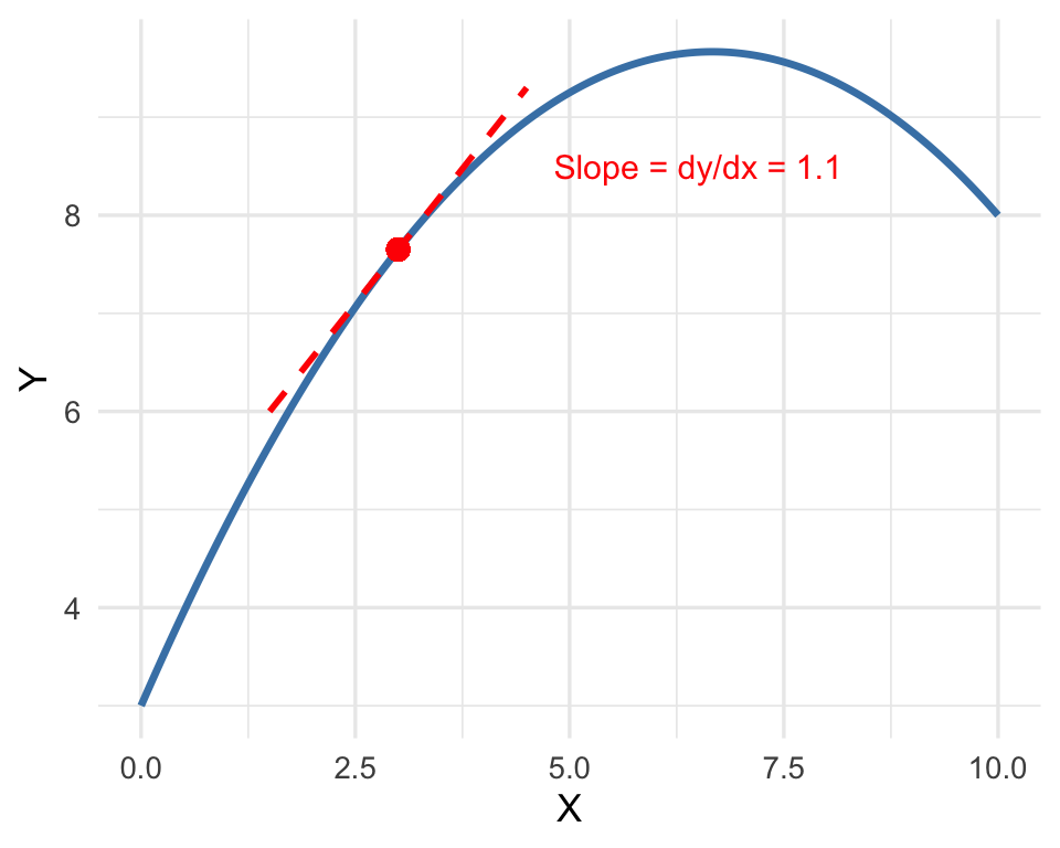
Visualizing Marginal Effects

The marginal effect is the instantaneous slope or the partial derivative of the regression surface

Categorical Moderators

An interaction can also involve a categorical variable.

Does the effect of studying differ by gender?

Now we’re asking if the slope for hours studied is different for males and females.

Visualizing Interaction by Gender

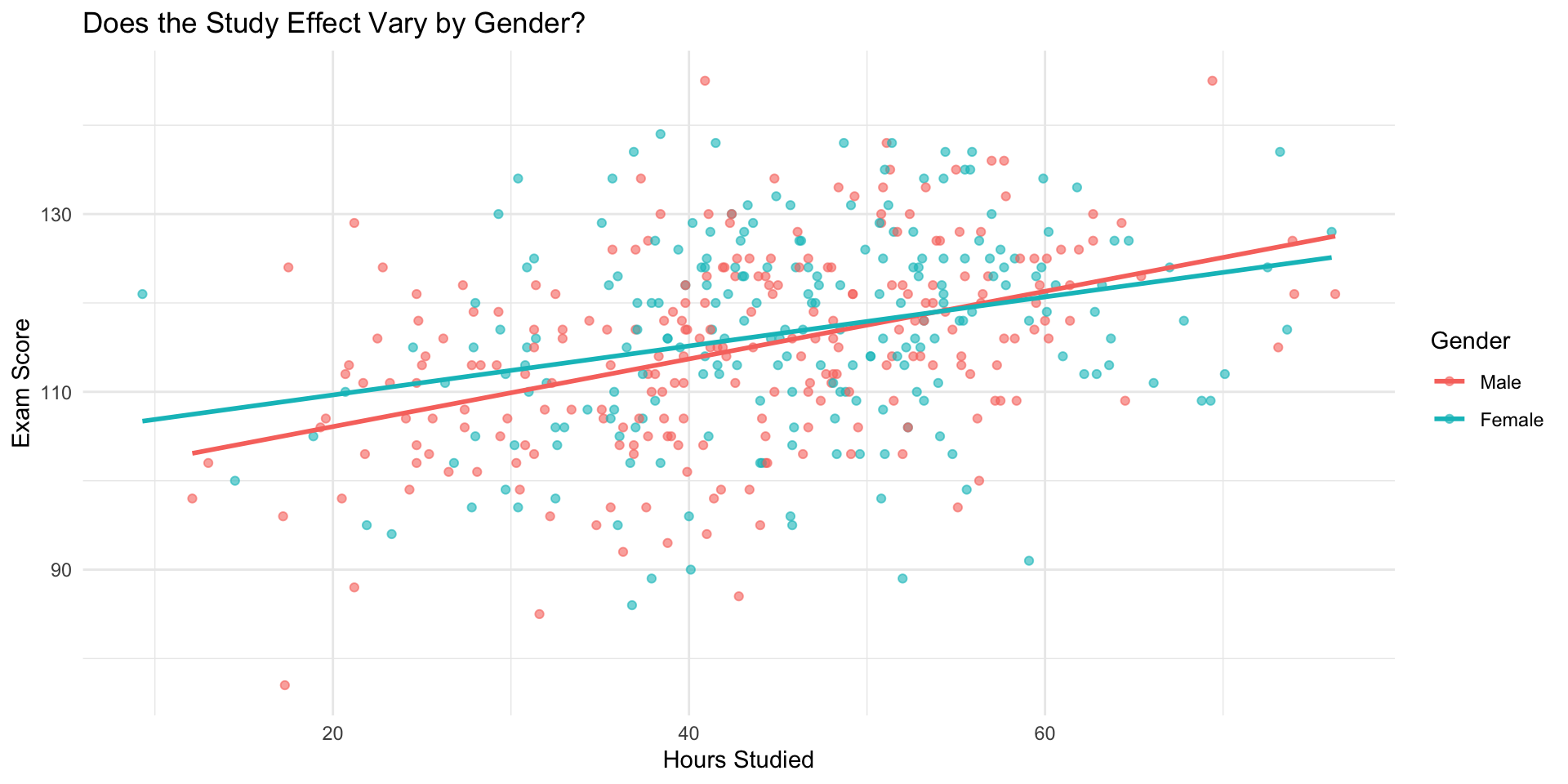
Model with Gender Interaction

mod_gender_interact <- lm(exam_score ~ hours_studied * gender, data = data)
summary(mod_gender_interact)


Call:
lm(formula = exam_score ~ hours_studied * gender, data = data)

Residuals:
     Min       1Q   Median       3Q      Max 
-29.4718  -6.7860   0.2575   6.8464  30.9571 

Coefficients:
                           Estimate Std. Error t value Pr(>|t|)    
(Intercept)                98.47665    2.37389  41.483  < 2e-16 ***
hours_studied               0.38059    0.05322   7.152 3.47e-12 ***
genderFemale                5.66051    3.73230   1.517    0.130    
hours_studied:genderFemale -0.10493    0.08062  -1.302    0.194    
---
Signif. codes:  0 '***' 0.001 '**' 0.01 '*' 0.05 '.' 0.1 ' ' 1

Residual standard error: 10.27 on 452 degrees of freedom
Multiple R-squared:  0.1448,    Adjusted R-squared:  0.1391 
F-statistic: 25.51 on 3 and 452 DF,  p-value: 2.914e-15

✅ This fits a different slope for males and females
✅ Also adjusts for any overall mean difference

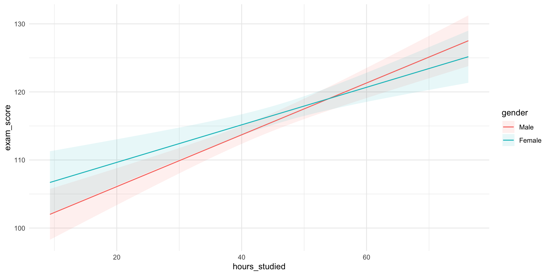
Model Equation (Gender Interaction)

The fitted model becomes:

\[ y = \beta_0 + \beta_1 \times \text{Hours} + \beta_2 \times \text{Female} + \beta_3 \times (\text{Hours} \times \text{Female}) \]

\(\beta_0\): mean exam score for males with \(0\) hours studied
\(\beta_1\): effect of studying for males (reference group)
\(\beta_2\): mean difference between genders when hours = 0
\(\beta_3\): difference in slope for females compared to males

Interpretation

For males (gender = 0):
➡️ Effect of studying is \(\beta_1\)
For females (gender = 1):
➡️ Effect of studying is \(\beta_1 + \beta_3\)

🧠 Interactions change the slope — not just the intercept

Visualizing Gender Interaction


 gender Estimate Std. Error    z Pr(>|z|)    S 2.5 % 97.5 %
 Male      0.381     0.0532 7.15   <0.001 40.1 0.276  0.485
 Female    0.276     0.0605 4.55   <0.001 17.5 0.157  0.394

Term: hours_studied
Type: response
Comparison: dY/dX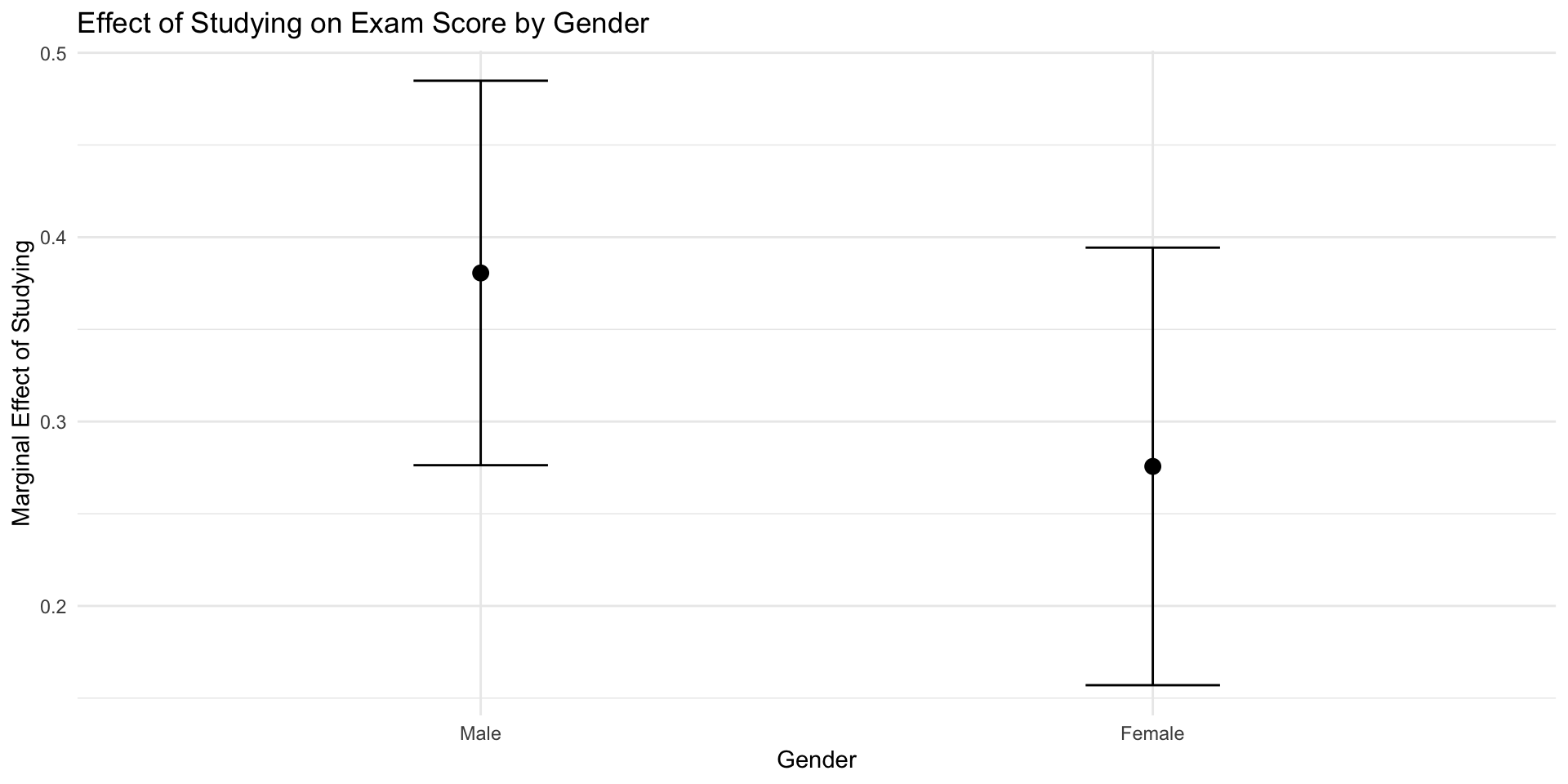

Predictions Visualized

mod <- lm(exam_score ~ hours_studied * gender, data = data)

# Get predictions for a grid of values
plot_predictions(mod,
  condition = list("hours_studied",
    "gender"
  )) + theme_minimal()

🔄 What We Learned About Interactions

Interactions (moderators) reveal effect heterogeneity:

The relationship between a predictor and the outcome varies across levels of another variable.

✅ Visual clue: Non-parallel lines in scatterplots or slope plots

✅ Statistical clue: Significant interaction term in the model

Types of Interactions:

🧮 Numeric × Numeric → slope changes continuously

👥 Categorical × Numeric → slope changes by group

👥 Categorical × Categorical → group differences depend on each other

Non-linear Associations

Why Non-linearities Matter

Not all relationships are straight lines.

Some effects diminish: each extra hour studied helps, but less and less.
Others accelerate: benefits appear only after a threshold.
Many real social relationships are curved, saturating, or U-shaped.

💡 In regression, we can capture this by including transformed variables,
like squared terms, logs, or polynomials.

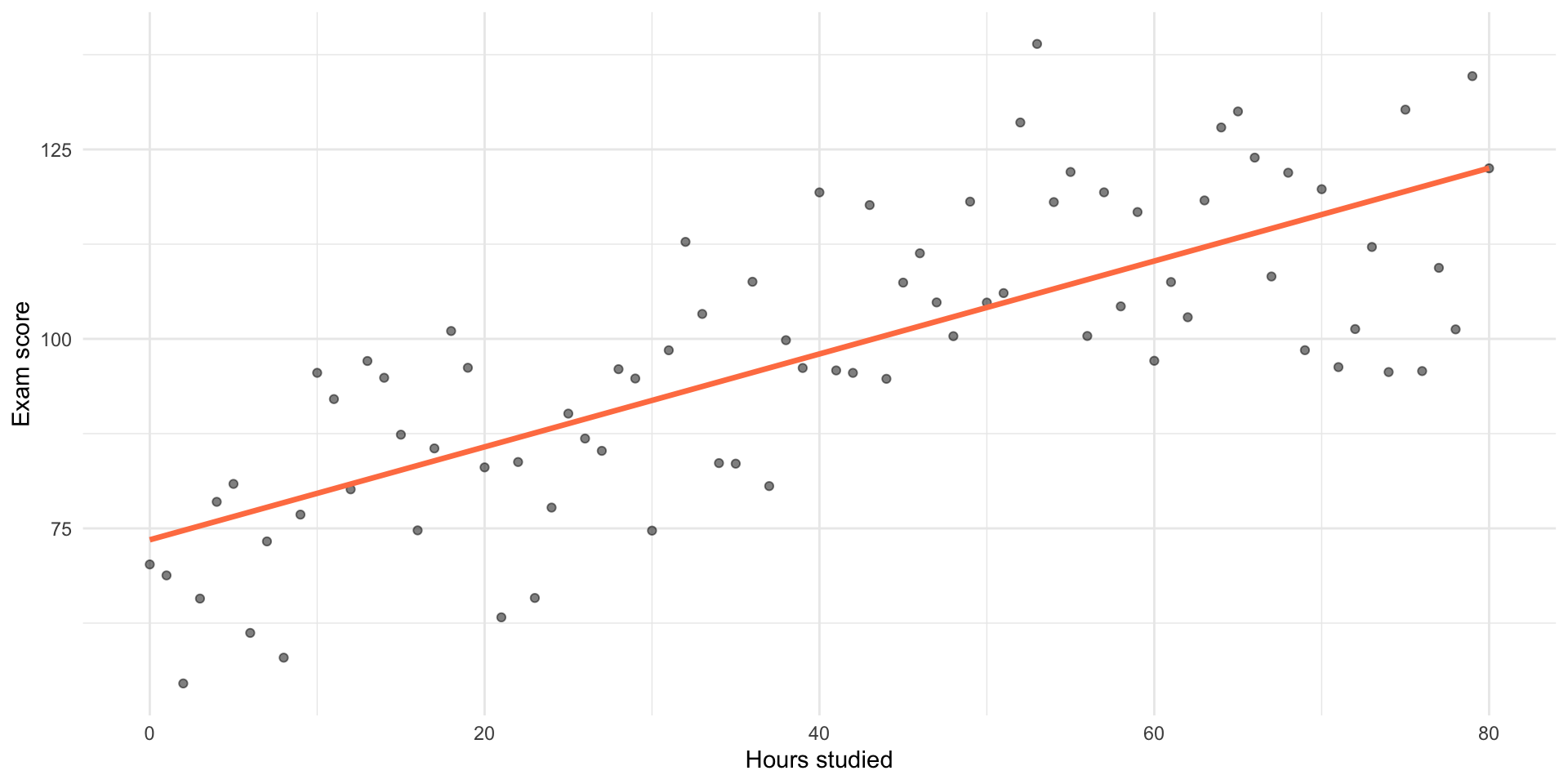
Example: Diminishing Returns to Studying

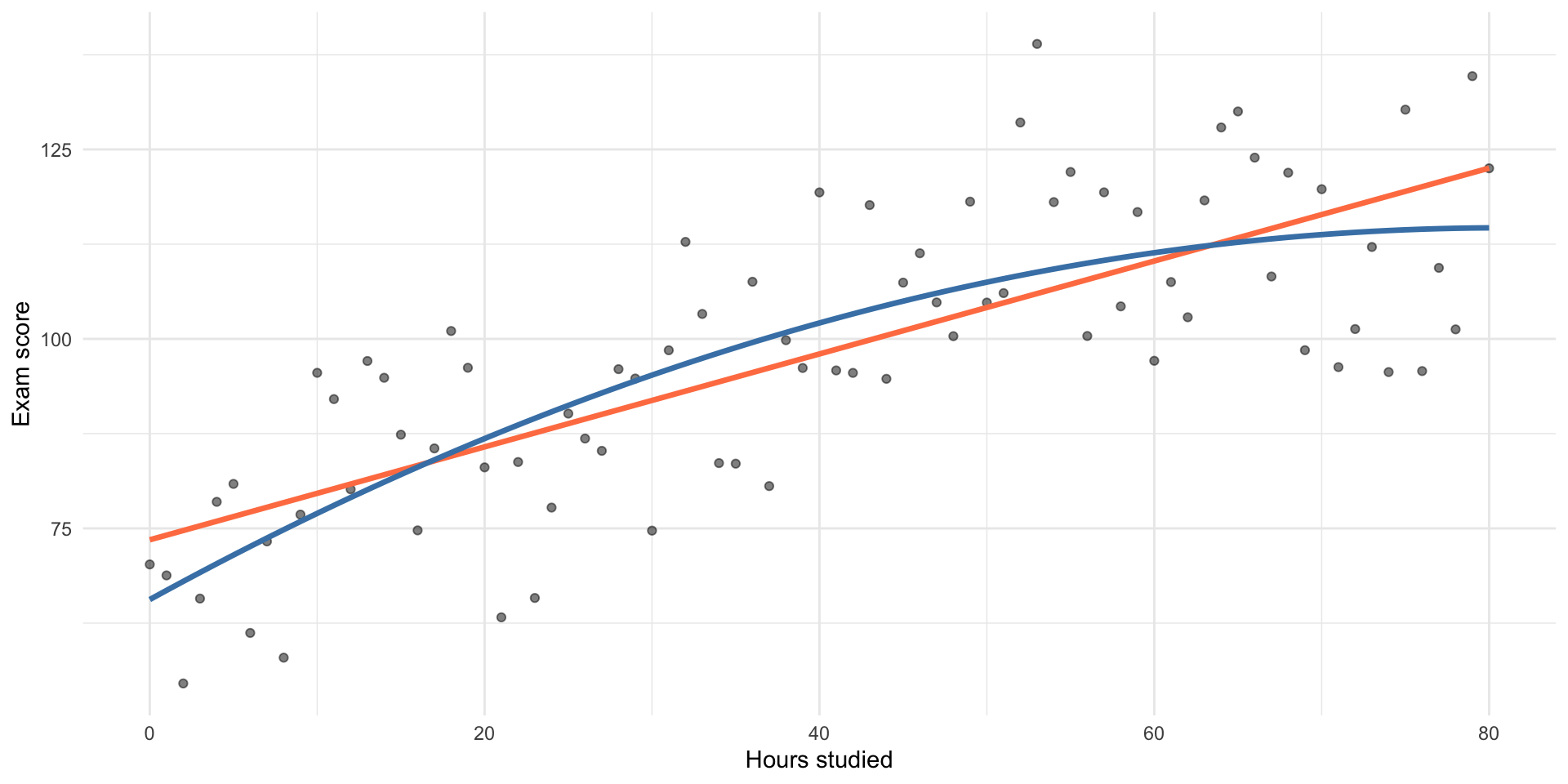
Adding a Squared Term

To model this curve, we can include \(x^2\):

\[ \widehat{y} = \beta_0 + \beta_1 x + \beta_2 x^2 \]

\(\beta_1\) → slope when \(x = 0\)
\(\beta_2\) → how fast the slope changes (curvature)
Same rule as for other interactions: You must include all the lower order terms
- e.g. if you include \(x^2\) you must include \(x\).
- if you include \(x^3\) you must include?
- if you include \(x \times z\) you must include?

Adding a Squared Term


Call:
lm(formula = score ~ hours + I(hours^2), data = d)

Residuals:
     Min       1Q   Median       3Q      Max 
-24.4906  -8.3426  -0.4449   8.8298  30.1122 

Coefficients:
             Estimate Std. Error t value Pr(>|t|)    
(Intercept) 65.610923   3.951576  16.604  < 2e-16 ***
hours        1.211540   0.228325   5.306 1.02e-06 ***
I(hours^2)  -0.007482   0.002761  -2.709  0.00828 ** 
---
Signif. codes:  0 '***' 0.001 '**' 0.01 '*' 0.05 '.' 0.1 ' ' 1

Residual standard error: 12.15 on 78 degrees of freedom
Multiple R-squared:  0.6062,    Adjusted R-squared:  0.5961 
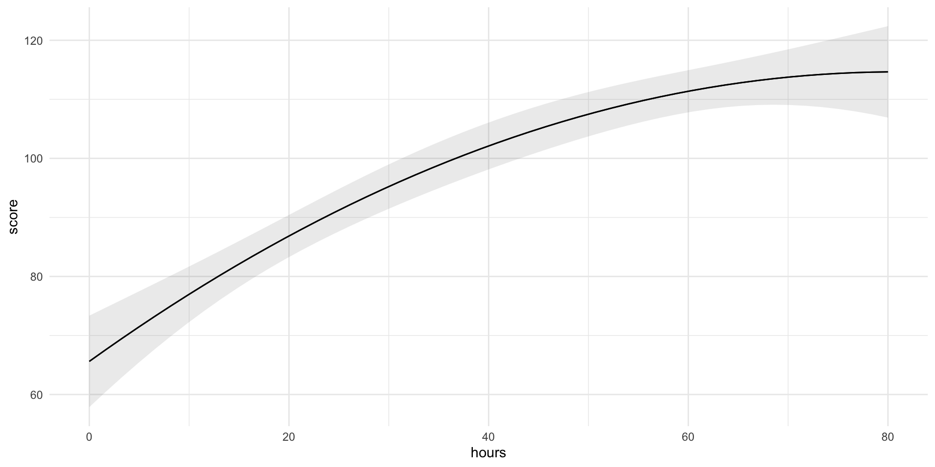
F-statistic: 60.04 on 2 and 78 DF,  p-value: < 2.2e-16

Interpreting a Squared Term

plot_slopes(
  mod_nonl,
  variables = "hours",
  condition = "hours"
) + theme_minimal()

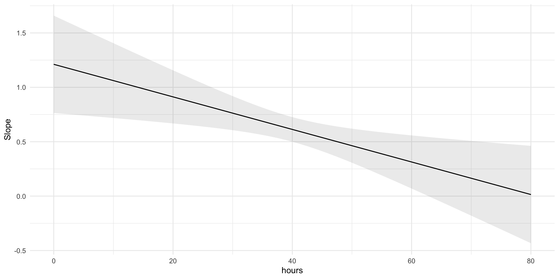
Interpreting a Squared Term

plot_predictions(
  mod_nonl,
  condition = "hours"
) + theme_minimal()

Other Common Transformations

Transformation	Example	Typical pattern captured	Interpretation
Quadratic	\(x^2\)	Curvature (U-shape or inverted-U)	Effect grows or shrinks with \(x\); marginal effect changes linearly
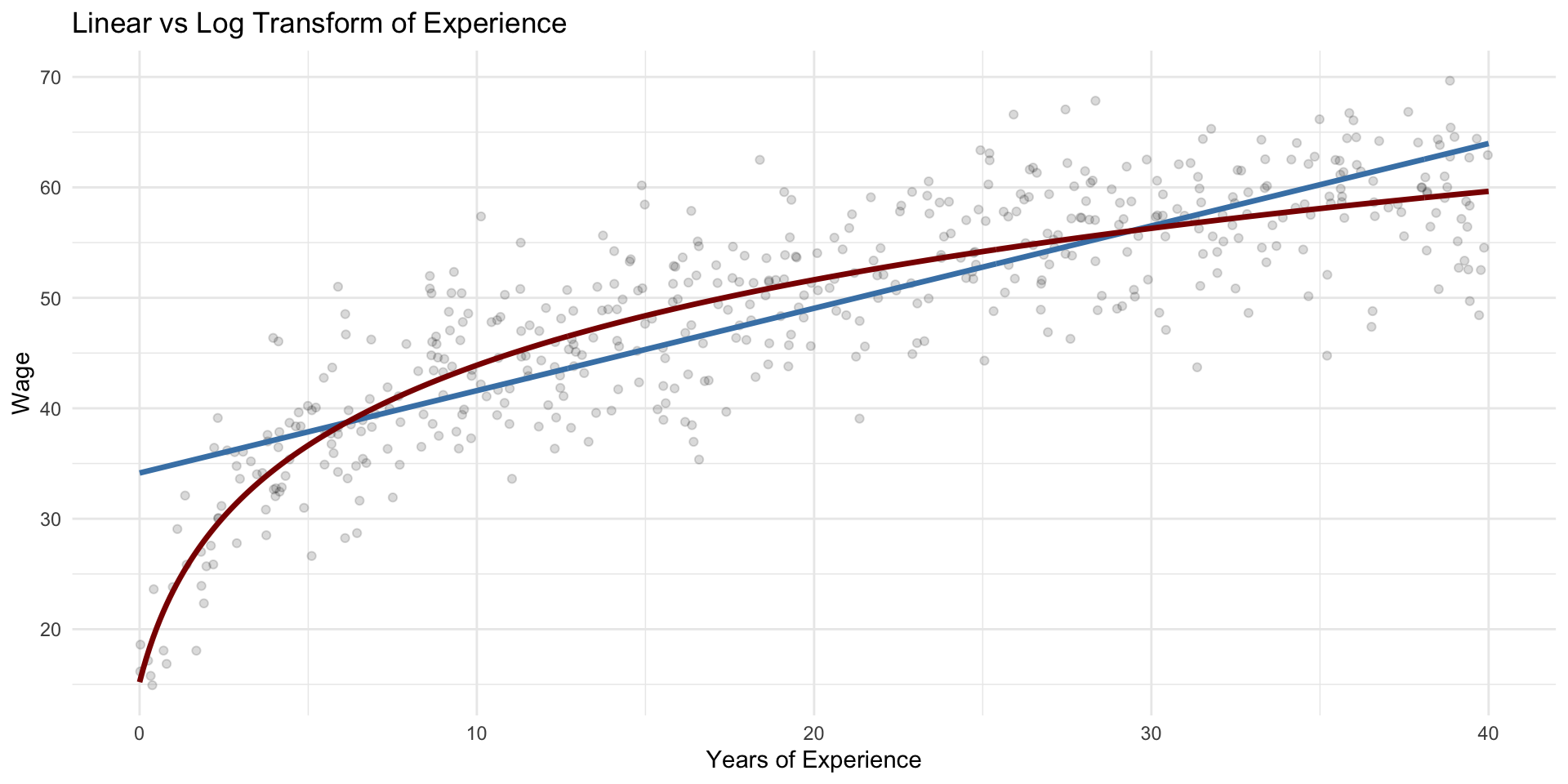
Logarithm of x	\(log(x)\)	Diminishing returns	A % change in \(x\) gives a constant change in \(y\)
Logarithm of y	\(log(y)\)	Multiplicative effects / skewed outcomes	Coefficients become semi-elasticities: 1-unit change in \(x\) → %Δ in \(y\)

Transformations reshape the functional form

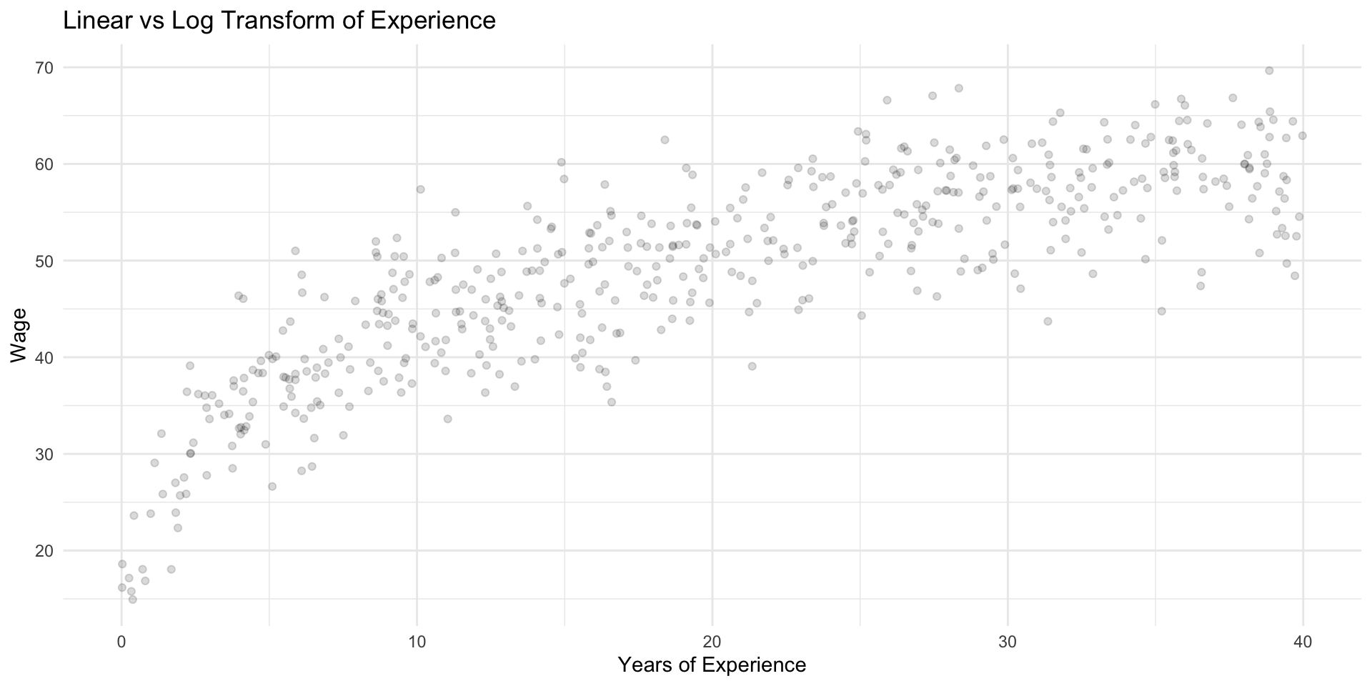
Squared vs Log Transform: Shape of the Relationship

Units

Units and Interpretation

mod <- lm(exam_score ~ hours_studied + previous_gpa, data = data)


Call:
lm(formula = exam_score ~ hours_studied + previous_gpa, data = data)

Residuals:
     Min       1Q   Median       3Q      Max 
-27.6294  -5.5828   0.2299   5.3861  26.1088 

Coefficients:
              Estimate Std. Error t value Pr(>|t|)    
(Intercept)   76.52508    2.10517   36.35  < 2e-16 ***
hours_studied  0.21709    0.03269    6.64 8.98e-11 ***
previous_gpa   0.40547    0.02545   15.93  < 2e-16 ***
---
Signif. codes:  0 '***' 0.001 '**' 0.01 '*' 0.05 '.' 0.1 ' ' 1

Residual standard error: 8.234 on 453 degrees of freedom
Multiple R-squared:  0.4486,    Adjusted R-squared:  0.4462 
F-statistic: 184.3 on 2 and 453 DF,  p-value: < 2.2e-16

Note the coefficient for hours_studied and the \(R^2\)

Units and Interpretation

data <- data %>%
  mutate(workdays_studied = hours_studied / 8)
mod2 <- lm(exam_score ~ workdays_studied + previous_gpa, data = data)

What will happen to the \(\beta\) and to the \(R^2\)?


Call:
lm(formula = exam_score ~ workdays_studied + previous_gpa, data = data)

Residuals:
     Min       1Q   Median       3Q      Max 
-27.6294  -5.5828   0.2299   5.3861  26.1088 

Coefficients:
                 Estimate Std. Error t value Pr(>|t|)    
(Intercept)      76.52508    2.10517   36.35  < 2e-16 ***
workdays_studied  1.73669    0.26154    6.64 8.98e-11 ***
previous_gpa      0.40547    0.02545   15.93  < 2e-16 ***
---
Signif. codes:  0 '***' 0.001 '**' 0.01 '*' 0.05 '.' 0.1 ' ' 1

Residual standard error: 8.234 on 453 degrees of freedom
Multiple R-squared:  0.4486,    Adjusted R-squared:  0.4462 
F-statistic: 184.3 on 2 and 453 DF,  p-value: < 2.2e-16

Note the coefficient for workdays_studied and the \(R^2\)

Units and Interpretation

data <- data %>%
  mutate(workweeks_studied = hours_studied / 40)
mod3 <- lm(exam_score ~ workweeks_studied + previous_gpa, data = data)


Call:
lm(formula = exam_score ~ workweeks_studied + previous_gpa, data = data)

Residuals:
     Min       1Q   Median       3Q      Max 
-27.6294  -5.5828   0.2299   5.3861  26.1088 

Coefficients:
                  Estimate Std. Error t value Pr(>|t|)    
(Intercept)       76.52508    2.10517   36.35  < 2e-16 ***
workweeks_studied  8.68346    1.30769    6.64 8.98e-11 ***
previous_gpa       0.40547    0.02545   15.93  < 2e-16 ***
---
Signif. codes:  0 '***' 0.001 '**' 0.01 '*' 0.05 '.' 0.1 ' ' 1

Residual standard error: 8.234 on 453 degrees of freedom
Multiple R-squared:  0.4486,    Adjusted R-squared:  0.4462 
F-statistic: 184.3 on 2 and 453 DF,  p-value: < 2.2e-16

This is why this is crucial:

“…associated with a one-unit increase in (\(X_j\))…”

Centering

Centering is a simple transformation that helps with:

Interpretation – makes intercepts meaningful.
Numerical stability – reduces collinearity in interaction models.

Centering

We “center” a variable by subtracting its mean:

data <- data %>%
  mutate(hours_centered = hours_studied - mean(hours_studied, na.rm = TRUE))
data %>% dplyr::select(hours_studied, hours_centered) %>% head()

  hours_studied hours_centered
1          26.2     -18.200439
2          33.0     -11.400439
3          42.6      -1.800439
4          35.4      -9.000439
5          53.8       9.399561
6          62.9      18.499561

Centering

mod <- lm(exam_score ~ hours_studied + previous_gpa, data = data)
summary(mod)


Call:
lm(formula = exam_score ~ hours_studied + previous_gpa, data = data)

Residuals:
     Min       1Q   Median       3Q      Max 
-27.6294  -5.5828   0.2299   5.3861  26.1088 

Coefficients:
              Estimate Std. Error t value Pr(>|t|)    
(Intercept)   76.52508    2.10517   36.35  < 2e-16 ***
hours_studied  0.21709    0.03269    6.64 8.98e-11 ***
previous_gpa   0.40547    0.02545   15.93  < 2e-16 ***
---
Signif. codes:  0 '***' 0.001 '**' 0.01 '*' 0.05 '.' 0.1 ' ' 1

Residual standard error: 8.234 on 453 degrees of freedom
Multiple R-squared:  0.4486,    Adjusted R-squared:  0.4462 
F-statistic: 184.3 on 2 and 453 DF,  p-value: < 2.2e-16

Centering

mod <- lm(exam_score ~ hours_centered + previous_gpa, data = data)
summary(mod)


Call:
lm(formula = exam_score ~ hours_centered + previous_gpa, data = data)

Residuals:
     Min       1Q   Median       3Q      Max 
-27.6294  -5.5828   0.2299   5.3861  26.1088 

Coefficients:
               Estimate Std. Error t value Pr(>|t|)    
(Intercept)    86.16382    1.89758   45.41  < 2e-16 ***
hours_centered  0.21709    0.03269    6.64 8.98e-11 ***
previous_gpa    0.40547    0.02545   15.93  < 2e-16 ***
---
Signif. codes:  0 '***' 0.001 '**' 0.01 '*' 0.05 '.' 0.1 ' ' 1

Residual standard error: 8.234 on 453 degrees of freedom
Multiple R-squared:  0.4486,    Adjusted R-squared:  0.4462 
F-statistic: 184.3 on 2 and 453 DF,  p-value: < 2.2e-16

The slope (\(\beta_1\)) is unchanged.
The intercept now represents the expected exam score for a student with average study hours.
Especially useful before adding interaction terms.

Why it matters for interactions

When you include an interaction term:

\[ Y = \beta_0 + \beta_1 X_1 + \beta_2 X_2 + \beta_3 (X_1 \times X_2) \]

centering prevents the main effects (\(\beta_1, \beta_2\)) from being interpreted at unrealistic values (e.g., when both predictors = 0).

✅ Often good: Center continuous variables before testing interactions.
It does not change model fit or significance — only makes interpretation clearer and more stable.

🧠 Lecture 3 Wrap-Up: What You Now Know

🔁 Interactions

Show that effects can depend on other variables — the slope is not always constant
Can be numeric × numeric (e.g. GPA × hours) or categorical × numeric (e.g. gender × hours)
Represented as multiplicative terms in the model
Best understood through visualization or marginal effects

📈 Non-linear Relationships

Effects can also vary along a single variable — not just between groups
We can capture curvature with squared, log, or root transformations
The marginal effect is no longer constant — it changes with \(x\)

⚖️ Units and Interpretation

Regression coefficients always depend on the units of measurement
Scaling or transforming variables can change magnitude of coefficients,
and the fit or meaning of the model.
Centering continuous predictors (subtracting their mean) makes intercepts more meaningful
and helps when including interaction terms

Next week

We connect all this to causal reasoning
See you at the lab!