Avoids false precision: thresholds sometimes reflect reliable measurement.
Policy relevance: many decisions operate on cutoffs.
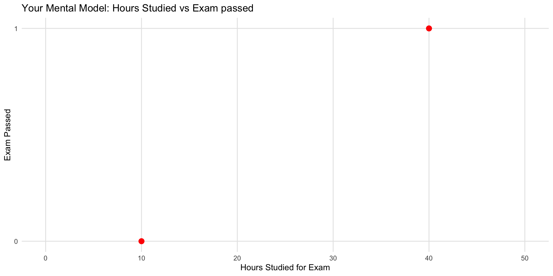
Key point:
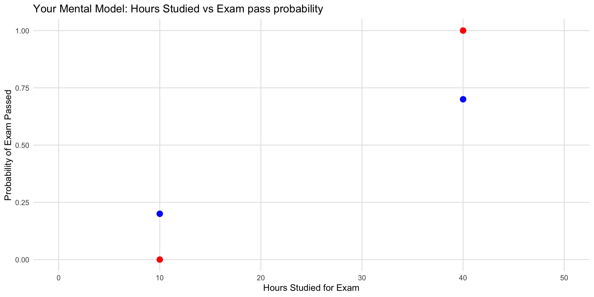
Today we’ll learn to model the probability that the event happens.
This is the backbone of logistic regression and most modern classification models.
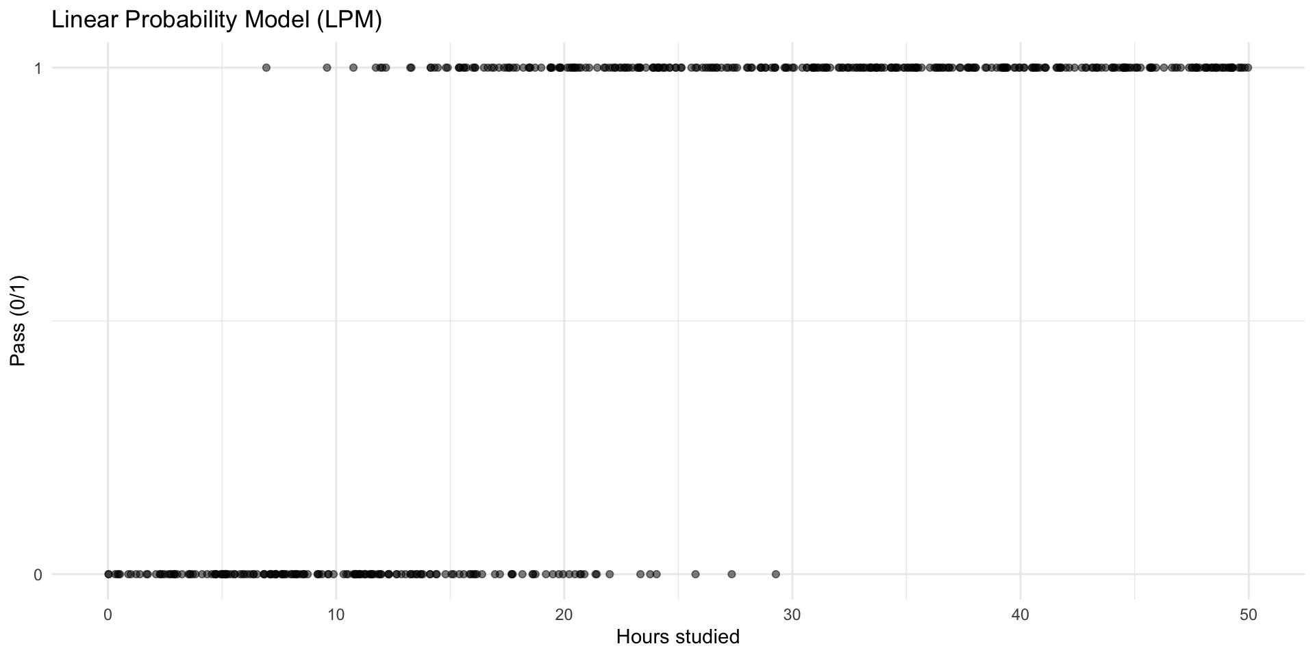
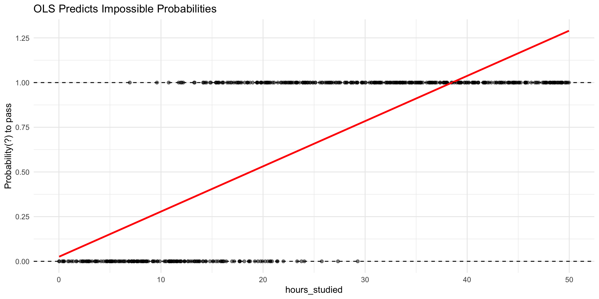
🔁 From OLS to the Linear Probability Model
We already know OLS can model a numeric outcome with a straight line.
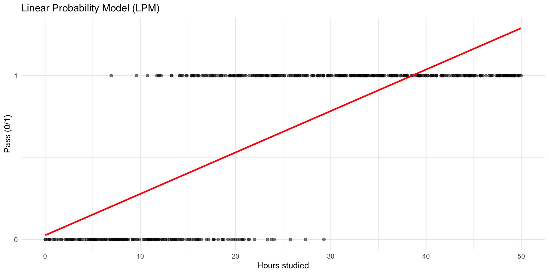
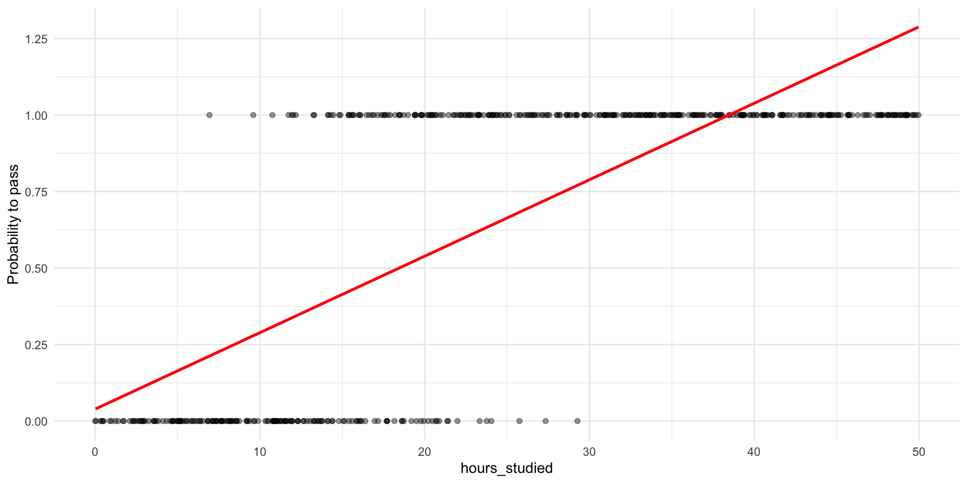
Linear Probability Model: treat 0/1 as numbers and run the same regression.
The slope can be interpreted as the change in probability with X.
In many cases, it works well enough for approximate answers.
But: the model is not a “true” probability model
Why Not Just Do Linear Probability Models?
💡 First, unreasonable probabilites
“What does a probability of 1.25 even mean? How could nature give you more than 100% chance?”
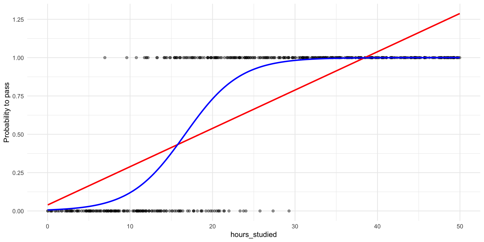
Second, incorrect funcional form
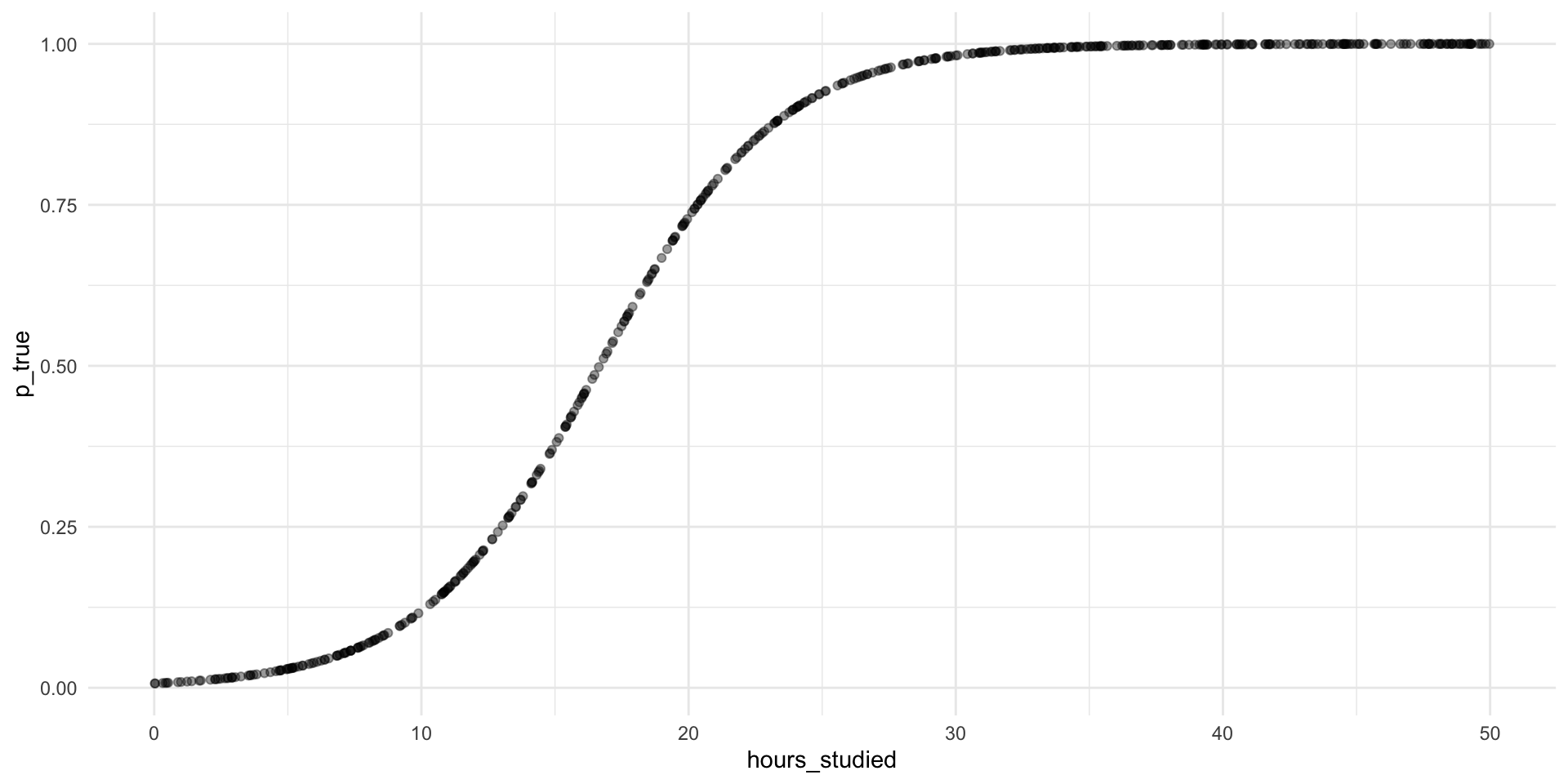
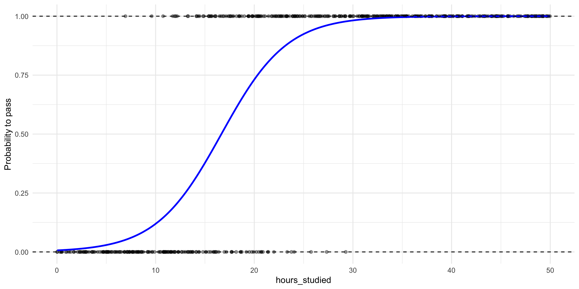
A more sensible shape for probabilities
What would you say about the marginal effect if we use a S-curve?
The change in \(p\) depends on where you are on the S-curve.
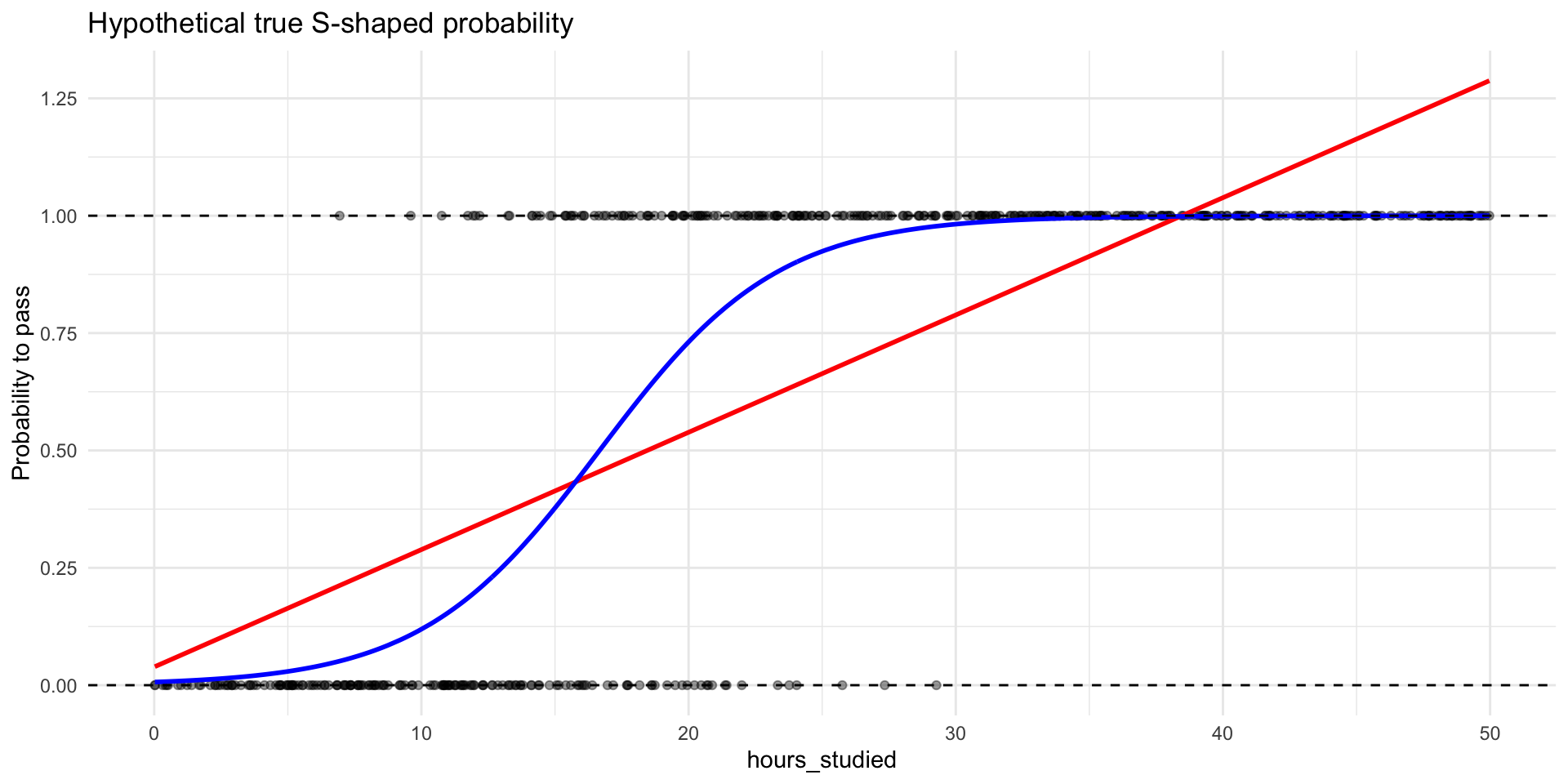
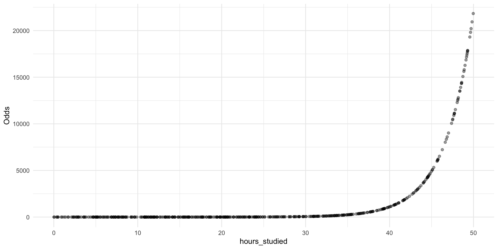
How do we model such a shape?
If we think the true relationship between \(X\) and the probability of \(Y=1\) has this S-shape, then we need a mathematical model that can produce that shape.
The plan is to find a way to transform the problem into something we already know how to do: Draw a straight line.
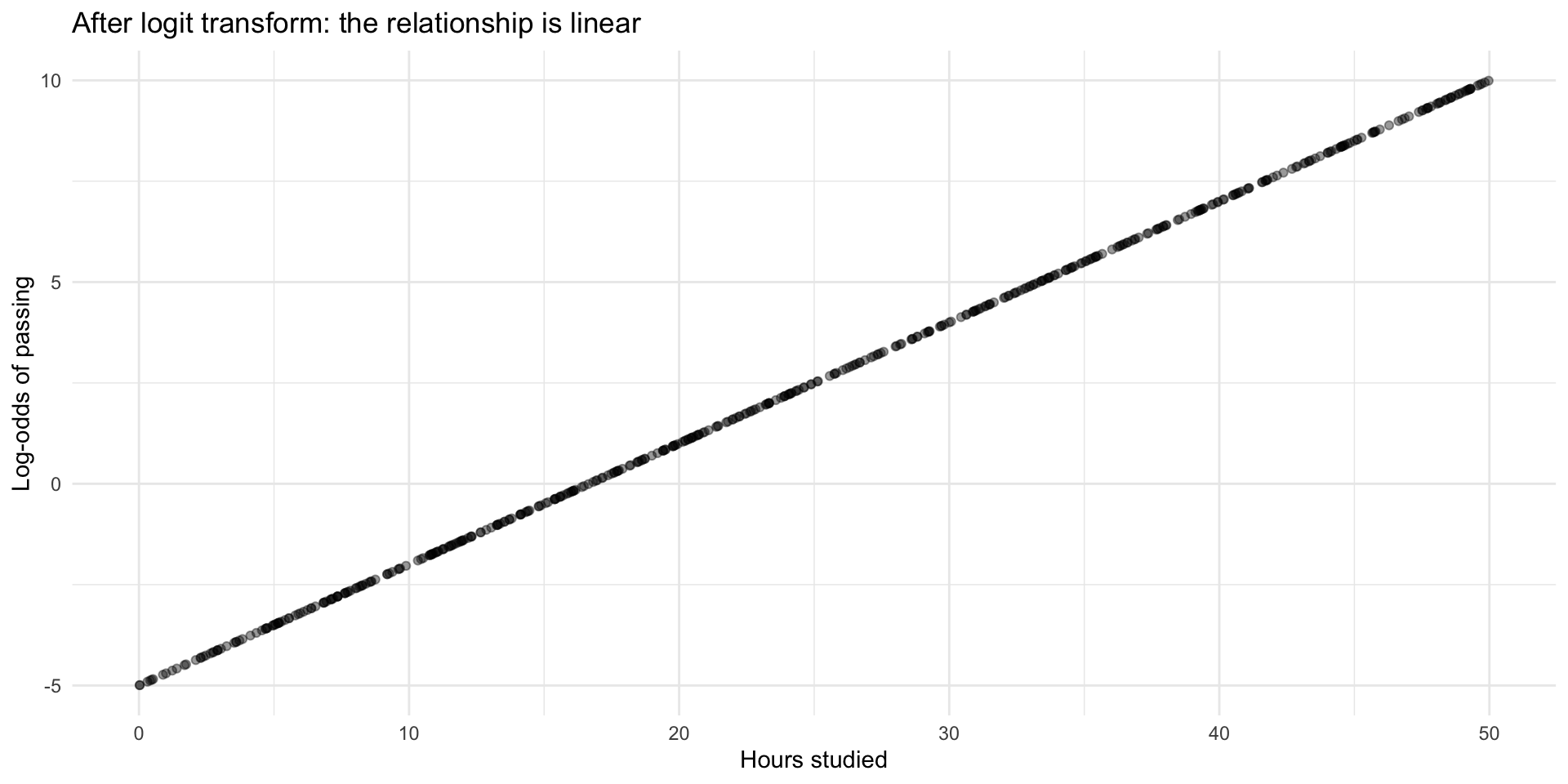
Let’s plot the log-odds against hours studied aaaaaaand….
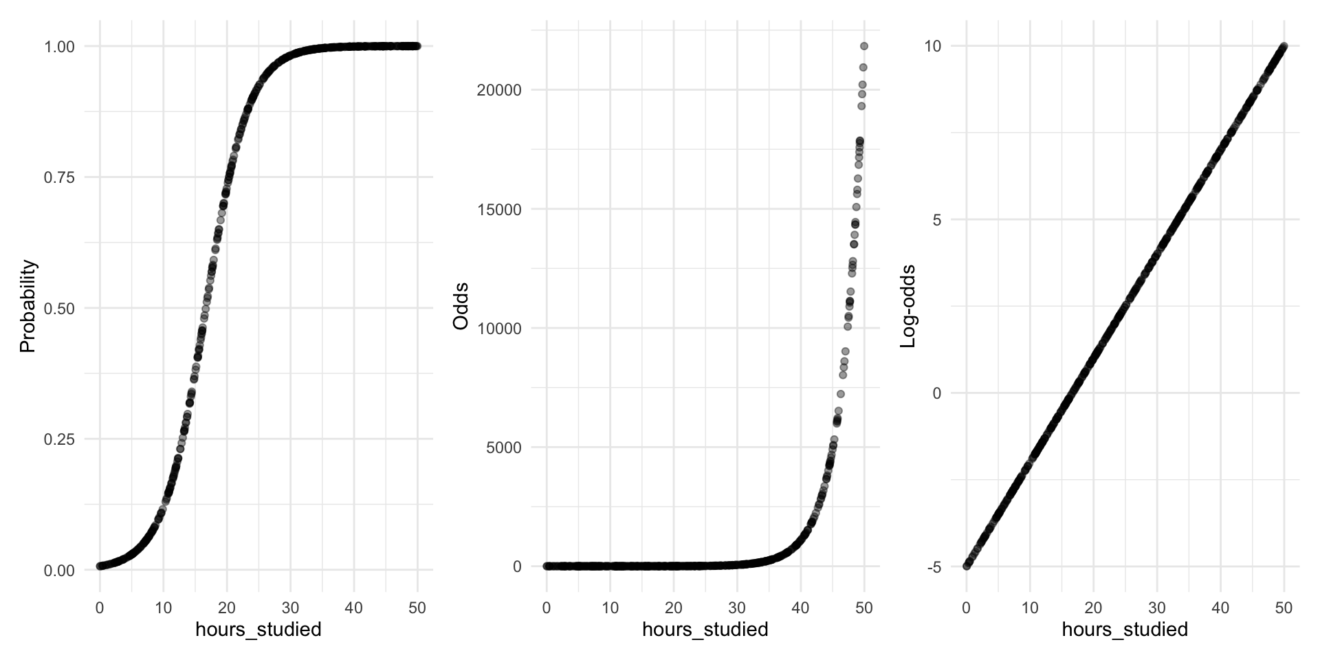
Transforming probabilities into something we can model
Summary
When the probability of (Y=1) follows an S-curve, the log-odds of (Y=1) follow a straight line
And a straight line we know how to model!
Logistic regression model
Great news! The log-odds can be modelled just like we are used to! \[\log(\text{odds}) = \beta_0 + \beta_1 X_1 + \beta_2 X_2 ... \]
Note: Log-odds can also be written \[\log(\text{odds}) = \log\left(\frac{p}{1-p}\right) = \text{logit}(p)\]
Let’s run a logistic regression
# New R function glm(): Generalized linear model# For logistic regression we have to specify `family = binomial`# (`family = gaussian` gives OLS)m1 <-glm(pass ~ hours_studied, family ="binomial", data = p_data)
Call:
glm(formula = pass ~ hours_studied, family = "binomial", data = p_data)

Coefficients:
              Estimate Std. Error z value Pr(>|z|)
(Intercept)   -5.21420    0.54485   -9.57   <2e-16 ***
hours_studied  0.30802    0.03073   10.02   <2e-16 ***
---
Signif. codes:  0 '***' 0.001 '**' 0.01 '*' 0.05 '.' 0.1 ' ' 1

(Dispersion parameter for binomial family taken to be 1)

    Null deviance: 646.20  on 499  degrees of freedom
Residual deviance: 228.92  on 498  degrees of freedom
AIC: 232.92

Number of Fisher Scoring iterations: 7
Intercept:
When hours_studied = 0, the estimated log-odds of passing are \(-5.21\).
Coefficient:
Each additional hour studied is associated with an increase of \(0.308\) in the log-odds of passing the exam, holding other variables constant.
It’s our friend the marginal effect! But in log-odds space.
Log-odds are not intuitive — what does “\(+ 0.3\) log-odds” mean?
Direction and uncertainty can still be interpreted.
💡 Towards better interpretation: Log-odds → Odds Ratios
💡 Towards better interpretation: Log-odds → Odds Ratios
💡 Towards better interpretation: Log-odds → Odds Ratios
\[
\log(\text{odds}) = \beta_0 + \beta_1 X
\]
Here, \(\beta_1\) is the additive effect on log-odds.
To get to odds, we exponentiate: \[
\text{exp}(\log(\text{odds})) = \text{odds} = \text{exp}(\beta_0 + \beta_1 X) = e^{\beta_0 + \beta_1 X}
\]
Intercept:
When hours_studied = 0, the estimated odds of passing are \(e^{\beta_0} = 0.005\).
Exponentiated coefficient:
Each additional hour studied multiplies the odds of passing by \(e^{\beta_1} = 1.36\) (i.e., about 36% increase in the odds per hour studied).
Important! Null-hypothesis is \(e^{\beta_1} = 1\)
\(x \times 1 = x\)
💡 Towards better interpretation: Probability marginal effects
Towards better interpretation: Probability marginal effects
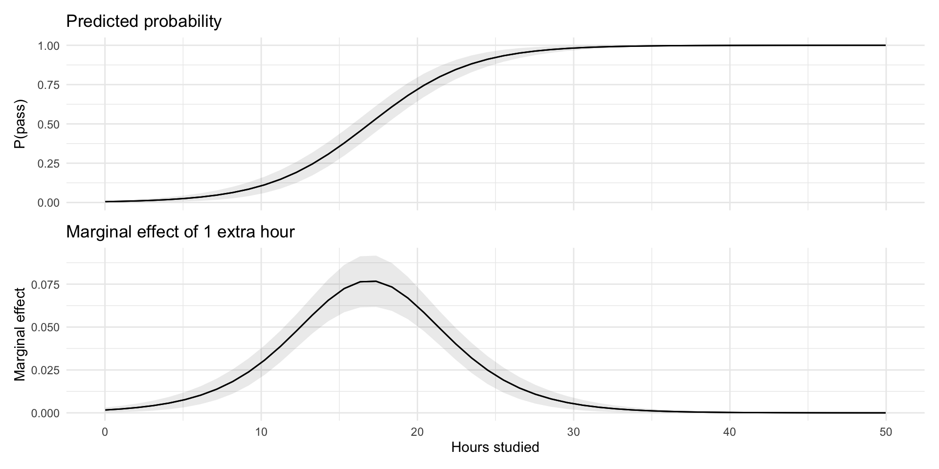
The change in \(p\) depends on where you are on the S-curve.
A bit like with non-linear relationships
Probabilities and Marginal Effects
The change in probability depends on where you are on the S-curve.
Largest at \(p = 0.5\) (middle of curve)
Smaller as \(p \to 0\) or \(p \to 1\)
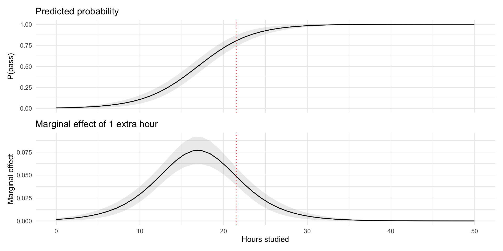
Probabilities and Marginal Effects
At 22h studied, the change in probability of passing the exam for a one-unit increase in hours studied is \(5\) percentage points, holding other variables constant.
Every predictor shifts the linear predictor → moves \(p\) to a different point on the S-curve.
Meaning, the level of every variable influences the marginal effect of any one variable.
🧠 Interpretation Challenge
For any predictor \(X_j\):
There is no universal “effect on probability.”
Individuals with different covariate profiles sit on different parts of the S-curve.
This variation is inherent to nonlinear models.
🧪 Hypothetical Cases
Like we’ve done before, consider a few concrete individuals:
Female, natural science, slept well, 20h study
Male, humanities, slept poorly, 10h study
Each hypothetical person will have a different effect of 1 additional hour of study, because their covariate values place them at different predicted probabilities.
🧮 Average Marginal Effects (AME)
If we can compute marginal effects for specific cases, we can compute them for every case in our sample.
AME does exactly this:
Compute the marginal effect of \(X_j\) for each observation \(i\).
Take the average.
Interpretation:
The AME tells us, on the probability scale, how much the outcome probability typically changes in this sample when X_j increases by one unit, taking into account that marginal effects differ across individuals.
📊 Why AMEs Work So Well
They operate on the probability scale → no log-odds translation.
They summarize heterogeneity across individuals.
They allow coefficient-style comparisons between variables.
They directly answer:
> “How much does this variable usually shift the predicted probability?”
AMEs give the most interpretable effect size in logistic regression.
🎯Model fit in logistic regression
🎯 Model Fit in Logistic Regression
Binary outcome → no continuous residuals
Two main angles:
Accuracy: How well predicted probabilities match outcomes
Classification: how often 0/1 is predicted correctly
Calibration: how predicted probabilities line up with actual proportions
Log likelihood measures: improvement over a null model
Pseudo-\(R^2\) (High values means better fit, but not the same as \(R^2\)!)
AIC and BIC (Low values better)
🧭 What to Look For
Reasonable probabilities
Any impossible or clearly implausible predictions?
Useful classification
Does a chosen cutoff make sense for your question?
Good calibration
Do predicted probabilities ≈ observed frequencies?
Better than the null model
Pseudo-R²: “How much better than predicting everyone the same?”
🔖 Summary
🤯 Stepping Back
Look at the path we’ve taken today:
Linear regression → breaks down for 0/1
Linear Probability Model → simple but “illegal” probabilities